Spatial growth-transform models

Introduction

The simplest mathematical models of neural networks are built from homogeneous McCulloch-Pitts neurons with scalar-weight connections between them. Biological neural networks, such as those in the mammalian cortex, are far more complex. They contain different types of neurons each with their own electrical behavior and spatially extended connections.

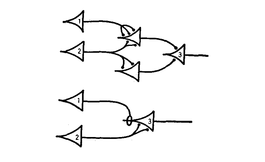
Example diagram of a simple neural network from the original 1943 paper by McCulloch and Pitts

A sample neural network diagram from the original 1943 paper by McCulloch and Pitts.

Computational neuroscientists standardly model biological neural networks as dynamical systems. Growth-transform (GT) models, introduced by Gangopadhyay and Chakrabartty, are one example. These models treat the change in membrane potential over time, \partial v/\partial t, as a growth-transform of the membrane potentials v on the net metabolic energy \mathcal{H} of a network, in the sense that it’s assumed that \partial v/\partial t satisfies the Baum-Eagon inequality: \mathcal{H}(v)\leq \mathcal{H}(v + \partial v/\partial t) In other words: \frac{\partial\mathcal{H}}{\partial v}\frac{\partial v}{\partial t} \leq 0 Thus, GT models are essentially energy-minimization models of neural dynamics.

In practical terms, instead of a one-dimensional weight between two homogeneous neurons, GT models use both a transconductance parameter and a temporal modulation factor to determine network behavior. Roughly, the transconductance parameter is the inverse of a traditional weight, while the temporal modulation factor allows for capturing the electrodynamics \partial v/\partial t of different neuron types at a single spatial point.

The GT models implemented in the DACx package add a third aspect of biological realism not captured by the original formulation of Gangopadhyay and Chakrabartty: a transmission velocity parameter for each neuron type. While the temporal modulation factor controls membrane voltage over time at a single spatial point, the transmission velocity parameter determines the rate at which changes in membrane voltage propagate between neurons. For this reason, we refer to our GT models as spatial GT (SGT) models.

SGT models thus allow for network topologies that not only capture connection strengths between neurons, but also the different types of neurons and their electrodynamics across both time and space. A separate tutorial demonstrates how to build network topologies for these models from circuit motifs. This tutorial explains SGT models in more detail.

Network nodes

Let’s set up the R environment by clearing the workspace, setting a random-number generator seed, and loading the DACx package.

# Clear the R workspace to start fresh
rm(list = ls())

# Set seed for reproducibility
set.seed(12345) 

# Load DACx package
library(DACx, quietly = TRUE)

Next, we create a new network object with the new.network function.

network.node <- new.network()

The object initialized by new.network is a minimal single-node network. In this context, “node” does not mean a single neuron, but rather a cluster of nearby neurons with local recurrent connections (e.g., see Park and Geffen, 2020). For this tutorial, our nodes will include three distinct neuron types: an excitatory type, layer 4 principal neurons (spiny stellates), and two inhibitory types, parvalbumin (PV) and somatostatin (SST) interneurons. These nodes are expected to be (approximately) fully connected, with cells of each type synapsing into cells of all other types.

Nodes are defined by their constitutive cell types and node size (expected number of neurons per type) and arrayed into layers and columns, mimicking the structure of the cortex. The network-topology tutorial provides more details on making layer-column structure. For now, it suffices to note that this structure is set with the set.network.structure function. We will set up a single-node network, with an expected count of 10 for the spiny stellates and 5 for each of the two inhibitory interneuron types.

network.node <- set.network.structure(
    network.node,
    neuron_types = c("spiny_stellate", "PV", "SST"),
    neurons_per_node = c(10, 5, 5)
  )

By default, the set.network.structure function sets the number of rows and columns each to one, i.e., makes a single node, and initializes local recurrent connections within that node. The node we just created can be visualized with the plot.network function. To keep the plot clean, we can use the arbor_density argument, which controls the proportion of cells for which the generated arbors are shown.

plt <- plot.network(network.node, arbor_density = 0.1)
plt$plot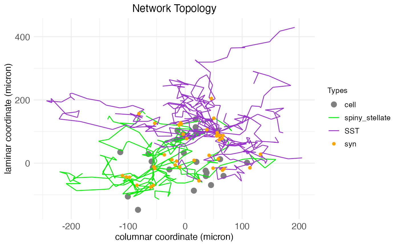

Here we see arbors for two cells, a spiny stellate and a SST interneuron. These arbors are generated via a biased random walk, the biasing factors fixed by cell type and controlling arbor shape. They include both axons and dendrites, which can be visualized explicitly by changing the arbor coloring. Although cells and arbors to-be-plotted are selected randomly, the plot.network function returns masks for the cells and arbors plotted, and can take this information to re-plot the same data again under different settings, e.g., coloring by arbor type instead of by cell type:

plt <- plot.network(
    network.node, 
    arbor_density = 0.1,
    soma_mask = plt$soma_mask,
    arbor_idx = plt$arbor_idx,
    edge_color = "is_axon"
    )
plt$plot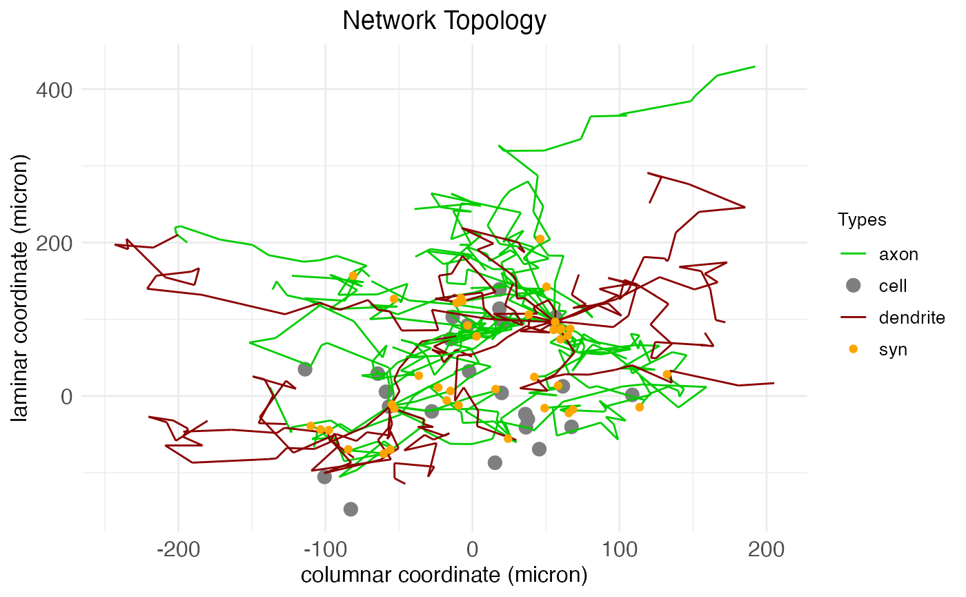

The existence and number of connections between cells – synapses, colored orange – are determined by the proximity of axons to dendrites. After the arbors are created, a separate algorithm looks for axon nodes within a certain small neighborhood of dendrite nodes and, if one is found, extends the axon to connect with the dendrite.

As the axis labels indicate, SGT models assign to each neuron a spatial coordinate giving its location along the laminar and columnar axes. While the above are 2D plots, there is in fact a third dimension, the “patch” dimension, which serves as a secondary columnar axis. All coordinates are continuous and real-valued and are used in conjunction with the transmission velocity parameter to simulate spike propagation over the axonal arbors. Here, for example, we can plot a 3D representation of our node including all arbors, colored by cell type:

plt <- plot.network(
    network.node, 
    arbor_density = 1.0,
    threedim = TRUE
  )
plt$plot

As can be seen, even for a small single node, the arborization and number of synapses can be extensive. We can quantify the extent by calling the fetch.network.components function, which returns a list of all components of the network, including a print out of summary data:

ntw <- fetch.network.components(network.node, include_arbors = TRUE)

## Summary of network: not_provided 
##  Number of neurons: 25 
##  Number of synapses: 386 
##  Layer names: layer 
##  Number of layers: 1 
##  Number of columns: 1 
##  Number of patches: 1 
##  Cell types used: spiny_stellate, PV, SST 
##  Motifs used: local connections

As the axis labels in the previous plots also indicate, there is a physically meaningful unit attached to the dimensions: microns. The actual control and setting of spatial coordinates is discussed in the network-topology tutorial.

Cell types

The three cell types (spiny stellates, PV, and SST) of the node are pre-defined in the neurons package. To see all cell types known by the package in the current session, we use the print.known.celltypes function:

print.known.celltypes()

## Known cell types:
## 
## Type: SST
##   Valence: -1
##   Temporal modulation bias (ms): 0.001
##   Temporal modulation time constant (ms): 0.001
##   Temporal modulation amplitude (ms): 0.003
##   Transmission velocity: 30000
##   Spine density: 0
##   Axon target: dendrite_shaft
##   Potential bound (mV): 75
##   Metabolic energy derivative dHdv bound (mA): 0.00105
##   Spike current (mA): 0.001
##   Spike potential (mV): 35
##   Resting potential (mV): -70
##   Threshold (mV): -55
##   Axon branch count: 10
##   Dendrite branch count: 10
##   Branch independence: 0.75
##   Branch spread: 0.75
##   Apical target layer: none
## 
## Type: PV
##   Valence: -1
##   Temporal modulation bias (ms): 0.001
##   Temporal modulation time constant (ms): 0.001
##   Temporal modulation amplitude (ms): 0
##   Transmission velocity: 30000
##   Spine density: 0
##   Axon target: soma
##   Potential bound (mV): 75
##   Metabolic energy derivative dHdv bound (mA): 0.00105
##   Spike current (mA): 0.001
##   Spike potential (mV): 35
##   Resting potential (mV): -70
##   Threshold (mV): -55
##   Axon branch count: 10
##   Dendrite branch count: 10
##   Branch independence: 0.625
##   Branch spread: 0.625
##   Apical target layer: none
## 
## Type: VIP
##   Valence: -1
##   Temporal modulation bias (ms): 0.0015
##   Temporal modulation time constant (ms): 0.001
##   Temporal modulation amplitude (ms): 0.0025
##   Transmission velocity: 30000
##   Spine density: 0
##   Axon target: dendrite_shaft
##   Potential bound (mV): 75
##   Metabolic energy derivative dHdv bound (mA): 0.00105
##   Spike current (mA): 0.001
##   Spike potential (mV): 35
##   Resting potential (mV): -70
##   Threshold (mV): -55
##   Axon branch count: 10
##   Dendrite branch count: 10
##   Branch independence: 0.625
##   Branch spread: 0.625
##   Apical target layer: none
## 
## Type: Neurogliaform_cell
##   Valence: -1
##   Temporal modulation bias (ms): 0.001
##   Temporal modulation time constant (ms): 0.001
##   Temporal modulation amplitude (ms): 0.001
##   Transmission velocity: 15000
##   Spine density: 0
##   Axon target: dendrite_shaft
##   Potential bound (mV): 75
##   Metabolic energy derivative dHdv bound (mA): 0.00105
##   Spike current (mA): 0.001
##   Spike potential (mV): 35
##   Resting potential (mV): -70
##   Threshold (mV): -55
##   Axon branch count: 10
##   Dendrite branch count: 10
##   Branch independence: 0.75
##   Branch spread: 0.75
##   Apical target layer: none
## 
## Type: spiny_stellate
##   Valence: 1
##   Temporal modulation bias (ms): 0.0015
##   Temporal modulation time constant (ms): 0.001
##   Temporal modulation amplitude (ms): 0
##   Transmission velocity: 30000
##   Spine density: 0.5
##   Axon target: spine
##   Potential bound (mV): 75
##   Metabolic energy derivative dHdv bound (mA): 0.00105
##   Spike current (mA): 0.001
##   Spike potential (mV): 35
##   Resting potential (mV): -70
##   Threshold (mV): -55
##   Axon branch count: 10
##   Dendrite branch count: 10
##   Branch independence: 0.75
##   Branch spread: 0.75
##   Apical target layer: none
## 
## Type: pyramidal_L6
##   Valence: 1
##   Temporal modulation bias (ms): 0.0035
##   Temporal modulation time constant (ms): 0.001
##   Temporal modulation amplitude (ms): 0
##   Transmission velocity: 30000
##   Spine density: 0.5
##   Axon target: spine
##   Potential bound (mV): 75
##   Metabolic energy derivative dHdv bound (mA): 0.00105
##   Spike current (mA): 0.001
##   Spike potential (mV): 35
##   Resting potential (mV): -70
##   Threshold (mV): -55
##   Axon branch count: 10
##   Dendrite branch count: 10
##   Branch independence: 0.25
##   Branch spread: 0.25
##   Apical target layer: L4
## 
## Type: pyramidal
##   Valence: 1
##   Temporal modulation bias (ms): 0.0035
##   Temporal modulation time constant (ms): 0.001
##   Temporal modulation amplitude (ms): 0
##   Transmission velocity: 30000
##   Spine density: 0.5
##   Axon target: spine
##   Potential bound (mV): 75
##   Metabolic energy derivative dHdv bound (mA): 0.00105
##   Spike current (mA): 0.001
##   Spike potential (mV): 35
##   Resting potential (mV): -70
##   Threshold (mV): -55
##   Axon branch count: 10
##   Dendrite branch count: 10
##   Branch independence: 0.25
##   Branch spread: 0.25
##   Apical target layer: L1

As can be seen from the output, cell types are defined by a number of parameters.

Cell type parameters

The parameters defining cell types in DACx are mostly biophysically interpretable and can be set with, or tested against, experimental data.

Parameters for transmitter type

Valence: 1 for excitatory cells, -1 for inhibitory cells. Code variable: valence.

Temporal modulation parameters

The temporal modulation term T controlling the responsiveness (size) of \partial v/\partial t is determined by an exponential decay function with parameters:

Temporal modulation bias: The baseline value b of T, in ms. Code variable: temporal_modulation_bias.
Temporal modulation time constant: The time constant \tau of the exponential decay in T, in ms. Code variable: temporal_modulation_timeconstant.
Temporal modulation amplitude: The amplitude A of the exponential decay in T, in ms. Code variable: temporal_modulation_amplitude. A value >0 induces bursting behavior, while a value of zero induces tonic (rhythmic) firing.

Development note: The values of these parameters are 1/0.0001 times the intended values in ms, due to debugging.

Intercell transmission parameters

Transmission velocity: The speed of the action potential between neurons, in microns/ms. Code variable: transmission_velocity.
Spine density: The proportion (a value between 0 and 1) of dendrite nodes expected to be spines. Code variable: spine_density.
Axon target: The kind of nodes onto which the cell’s axons can synapse. Possible values include “spine”, “dendrite_shaft”, “soma”, and “axon_shaft”. Code variable axon_target.

Membrane parameters

Potential bound: The maximum absolute value v_\mathrm{bound} of potential difference in electrical charge between the inside and outside of the cell, in mV. Code variable v_bound. Theoretically, we assume this is the absolute value of the rest voltage, plus a little bit. What matters is that -v_\mathrm{bound} \leq v \leq v_\mathrm{bound} for all possible membrane potentials v. For example, 75mV is a reasonable value.
Metabolic energy derivative bound: Bound \partial I_\mathrm{influx} on the absolute value of the derivative \partial\mathcal{H}/\partial v of metabolic energy \mathcal{H} with respect to potential v, such that \partial I_\mathrm{influx} \geq |\partial\mathcal{H}/\partial v|, in mA. Code variable: dHdv_bound. Theoretically, we assume that this value is approximately the change in current when v crosses the spike threshold, which we assume is approximately the spike current. In practice, we add 5%.
Spike current: The current of the action potential, i.e., the total current crossing the membrane over the entire area of the cell during a spike, in mA. Code variable: I_spike. As a starting point, we assume this is 10^{-3}mA, i.e., one mico amp.
Spike potential: The value v_\mathrm{spike} of an action potential, in mV. Code variable: spike_potential. The default is 35mV.
Resting potential: The potential difference v_\mathrm{rest} in electrical charge between the inside and outside of the cell at rest, in mV. Code variable: resting_potential. The default is -70mV.
Threshold: The potential difference v_\mathrm{threshold} in electrical charge between the inside and outside of the cell at which an action potential is triggered, in mV. Code variable: threshold. The default is -55mV.

Parameters for process size and structure

Axon branch count: An integer value giving the expected number of nodes per branch in the axon arbor. Code variable: axon_branch_count.
Dendrite branch count: Same as axon branch count, but for dendrites. Code variable: dendrite_branch_count.
Branch independence: The expected proportion (a value between 0 and 1) of branches which connect directly to the soma, with 1 meaning all branches connect directly to the soma and zero meaning that all branches connect to the soma from a single segment. Code variable: branch_independence.
Branch spread: Scaled value between 0 and 1 controlling the tendency of arbor branches to repel away from the soma with 1 meaning a straight line away from the soma and 0 meaning no bias with respect to soma position. Code variable: branch_spread.

Apical dendrite parameters

Apical target layer: Character string giving the name of the layer to which apical dendrite is expected to grow, if any; if none, “none”. Intended for modeling the circuit topology of pyramidal neurons. Code variable: apical_target_layer.

Synaptic conductance

There is one important cell-type property not controlled directly through the cell_type structure: synaptic conductance. Synaptic conductance is the ease with which current flows into a synapse, and thus represents synaptic “strength”. Of course, the strength of any one synapse is determined by a history of activity – or, from a modeling point of view, training. However, these values need to be initialized in some way and we can expect certain combinations of cell type, layer, and projection to be biased in certain directions for synaptic strength. These initialization biases are controlled through arguments in the set.network.structure function and the load.projection.into.motif function. The former controls synaptic conductance biases within nodes (local connections) and the latter controls synaptic conductance biases between nodes (meso-scale connections). In both cases, the value is specified in millisiemens (mS) and is set to 10^{-10}mS by default, which is equivalent to a 5 pico amp synaptic current at a 50mV potential.

Modifying cell types

Cell types themselves are technically a C++ struc. Defined cell types are stored in an unordered map in C++ that’s accessible via three R wrapper functions. The function add.cell.type can be used to add a new cell type to the map. The function modify.cell.type can be used to modify an existing cell type. The function fetch.cell.type.params will return the parameters of the named cell type as an R list.

Principal neurons

The DACx package includes a special cell type, “principal”, which can be called as well. This call doesn’t refer to any predefined cell type, but instead triggers a layer-dependent lookup of known principal cell types. The term “principal” simply means the primary cell type in a region. We can see known principal cell types by calling the principal.neurons function:

principal.neurons(print_nicely = TRUE)

## Principal neuron types by layer:
##   layer: spiny_stellate
##   L1: Neurogliaform_cell
##   L2: pyramidal
##   L3: pyramidal
##   L4: spiny_stellate
##   L5: pyramidal
##   L6: pyramidal_L6

As can be seen, spiny stellates are the principal cell for layer 4. We have used them for this demonstration because, unlike pyramidal cells, they do not extend apical dendrites out of their home layer.

SGT simulations

The function run.SGT runs a simulation of spiking activity across a network using a SGT model. The function is just a wrapper over the SGT method of C++ network objects. It takes three arguments:

network: A network created by the new.network function and structured by the set.network.structure function.
stimulus_current_matrix: A matrix of input currents (in mA) over the duration of the simulation, rows representing neurons and columns representing time bins.
dt: Time-step size for simulation, in ms. Default is 10^{-3}.

The number of columns of stimulus_current_matrix determines the length of the simulation. In essence, the function run.SGT answers the question: How would the network respond to this stimulus current over this amount of time?

For example, let’s create a 50ms simulation for the node we created above. From the above call to fetch.network.components, we know there are 25 neurons in our network. We can load this value directly from the function output:

n_neurons <- ntw$n_neurons

This gives us the number of rows needed in our stimulus current matrix. For the number of columns, we need to know the number of time steps required:

stim_time_ms <- 50
dt <- 1e-3
n_steps <- stim_time_ms/dt
cat("Number of time steps in the simulation:", n_steps)

## Number of time steps in the simulation: 50000

Now, suppose we want our simulation to involve a 20ms input current to just the spiny stellates, starting at 10ms. We can compute the initial and final time steps of this current, plus a mask for the spiny stellates, as follows:

# Set stimulus start and length
stim_length_ms <- 20
stim_start_ms <- 10
# Find start and end steps of the input stimulus current
stim_length <- stim_length_ms / dt
stim_start <- stim_start_ms / dt 
stim_end <- stim_start + stim_length - 1
# Find mask for principal neurons
spiny_stellate_mask <- ntw$neuron_type_name == "spiny_stellate"

A final question is how much current to apply. For this simulation, we’ll use a constant current of 100 pico amp (100\times 10^{-9}mA) to the spiny stellates during the stimulus period. It might be natural to leave the input current at zero outside of the stimulus period, but there is endogenous background activity even without exogenous input to the network. So, we’ll specify a baseline input current of 10 pico amps (10\times 10^{-9}mA) to all neurons throughout the entire stimulation period:

rest_current <- rnorm(n_neurons * n_steps, 0, 10 * 1e-9) # 10 pico amp expected
stimulus_current_matrix <- matrix(rest_current, nrow = n_neurons, ncol = n_steps)
stimulus_current_matrix[spiny_stellate_mask, stim_start:stim_end] <- stimulus_current_matrix[spiny_stellate_mask, stim_start:stim_end] + 100 * 1e-9 # ten pico amps

With the stimulus current matrix in hand, we can run the simulation:

sim_results <- run.SGT(
    network.node,
    stimulus_current_matrix,
    dt
  )

The result of the function run.SGT is a matrix of spike traces formatted similar to stimulus_current_matrix: each row represents a neuron and each column represents a time step from the simulation. Each entry is the membrane potential of the neuron at that time bin, in mV. The order of neurons and time steps matches across the input stimulus-current and output spike-trace matrices, of course. In addition, a vector of spike counts for each neuron (giving the number of times each neuron spiked) in the network is also returned. Both are returned in a list of two elements, sim_traces and spike_counts.

We can view the head of the simulation traces:

print(sim_results$sim_traces[1:10,1:10])

##       [,1]      [,2]      [,3]      [,4]      [,5]      [,6]      [,7]      [,8]      [,9]     [,10]
##  [1,]  -70 -69.99908 -69.99814 -69.99728 -69.99628 -69.99539 -69.99455 -69.99364 -69.99274 -69.99180
##  [2,]  -70 -69.99951 -69.99899 -69.99856 -69.99806 -69.99751 -69.99706 -69.99672 -69.99631 -69.99589
##  [3,]  -70 -69.99909 -69.99826 -69.99731 -69.99642 -69.99558 -69.99475 -69.99386 -69.99299 -69.99216
##  [4,]  -70 -69.99922 -69.99842 -69.99781 -69.99723 -69.99658 -69.99587 -69.99522 -69.99455 -69.99396
##  [5,]  -70 -69.99949 -69.99878 -69.99811 -69.99729 -69.99668 -69.99597 -69.99532 -69.99461 -69.99403
##  [6,]  -70 -69.99922 -69.99834 -69.99765 -69.99695 -69.99621 -69.99544 -69.99461 -69.99387 -69.99306
##  [7,]  -70 -69.99935 -69.99859 -69.99794 -69.99727 -69.99653 -69.99571 -69.99503 -69.99426 -69.99345
##  [8,]  -70 -69.99944 -69.99894 -69.99834 -69.99778 -69.99727 -69.99672 -69.99622 -69.99573 -69.99522
##  [9,]  -70 -69.99919 -69.99845 -69.99766 -69.99694 -69.99626 -69.99556 -69.99472 -69.99397 -69.99329
## [10,]  -70 -69.99924 -69.99840 -69.99761 -69.99685 -69.99612 -69.99536 -69.99460 -69.99379 -69.99291

As well as the head of the spike counts:

print(head(sim_results$spike_counts))

## [1] 9 5 9 7 7 8

The neurons package also includes the function plot.network.traces, which takes a network object with a trace matrix and produces a plot of the traces, putting all neurons of the same type together.

plot.network.traces(network.node)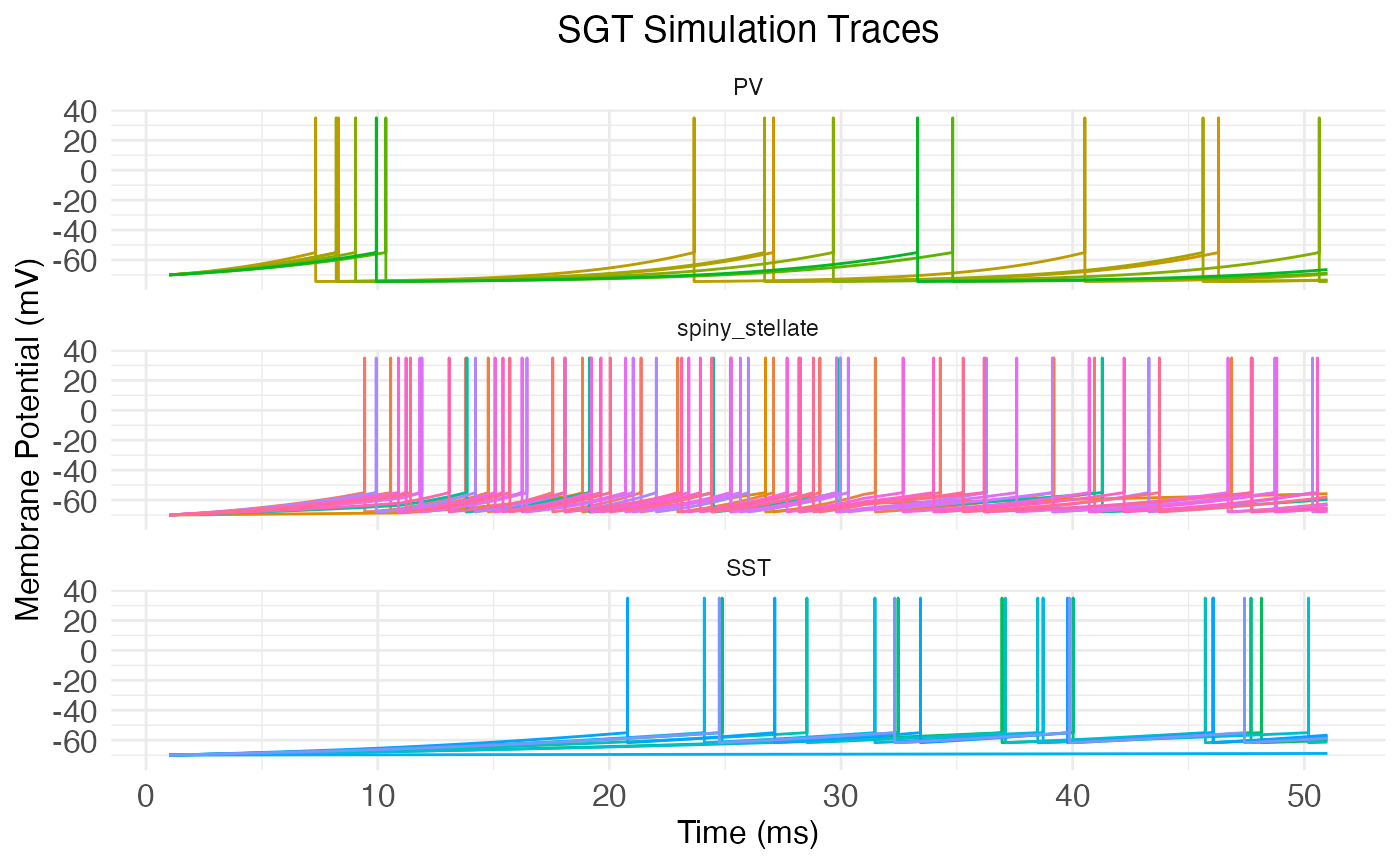

We can manually add the start and end of the stimulus period to the plot with vertical lines:

plt <- plot.network.traces(network.node, return_plot = TRUE)  +
  ggplot2::geom_vline(xintercept = stim_end * dt, linewidth = 1) +
  ggplot2::geom_vline(xintercept = stim_start * dt, linewidth = 1)
print(plt)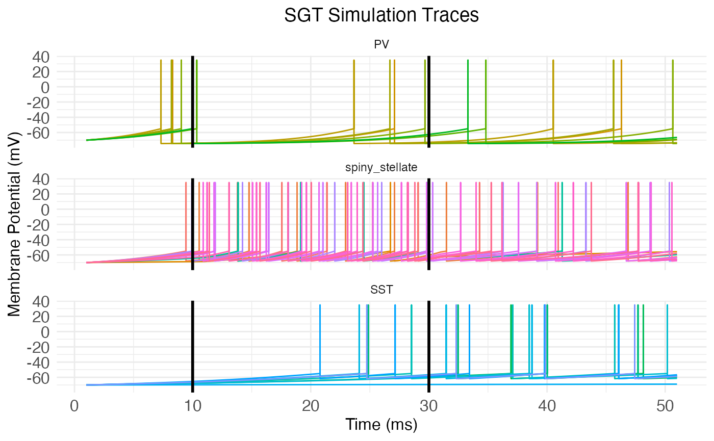

Mathematics of SGT models

GT models are hybrids, in so far as they directly model subthreshold membrane potential dynamics, while leaving out any mechanistic modeling of spikes themselves. Instead, spikes are modeled as a constant and instantaneous value v_\mathrm{spike} (variable spike_potential in the simulation) added to the subthreshold dynamics when the spike threshold is crossed. Thus, what follows is an explanation of the subthreshold component of membrane potential v, although we leave the qualifier “subthreshold” implicit.

Suppose our network has n neurons N. We want to run a simulation of the membrane potential v(t) of each neuron N over time t. Naturally, the system evolves so that: v(t+1) = v(t) + \left.\frac{\partial v}{\partial t}\right|_{t+1} The hard part, of course, is to compute \partial v/\partial t. That is, how do membrane potentials evolve over time? Gangopadhyay and Chakrabartty answered this question by applying the Baum-Eagon inequality to \mathcal{H} on v to derive \partial v/\partial t as a growth-transform. This amounts to assuming that net metabolic power \mathcal{H} is minimized over time. In this section, we will work directly from this minimization assumption and use a biologically inspired interpretation of the variables.

Power minimization

GT models tackle this question with a minimization principle: \partial v/\partial t is always such that the system minimizes net (metabolic) power \mathcal{H}: \frac{\partial\mathcal{H}}{\partial v}\frac{\partial v}{\partial t} \leq 0 For simplicity, let us assume that \partial\mathcal{H}/\partial t = 0, i.e., that the metabolic power is not changing over time.

It’s plausible that the membrane potential v is a scalar multiple fv_\mathrm{rest} of the resting potential v_\mathrm{rest}, where the scale factor f is a function of \partial\mathcal{H}/\partial v. In other words, we assume that the scale factor f depends on how a small change \partial v in membrane potential would change the metabolic power \mathcal{H}. Hence, we have that: v(t+1) = v(t) + \left.\frac{\partial v}{\partial t}\right|_{t+1} = f\left(\left.\frac{\partial\mathcal{H}}{\partial v}\right|_{t+1}\right)v_\mathrm{rest} Actually, in practice Gangopadhyay and Chakrabartty assume that the quantity of which v is a multiple is a positive value v_\mathrm{bound}. The only constraint on this value is that it must bound v from above and below, i.e., -v_\mathrm{bound} \leq v \leq v_\mathrm{bound}. Thus, it would be more mathematically accurate to say that v is a scalar multiple of the absolute value of v_\mathrm{rest}. Within the simulation code, the relevant variable is v_bound with a default value of 85 mV, slightly higher than the absolute value of v_\mathrm{rest}.

Scale factor

Therefore, if we could find a suitable scale factor f, we’d be able to compute \partial v/\partial t as: \left.\frac{\partial v}{\partial t}\right|_t = f\left(\left.\frac{\partial\mathcal{H}}{\partial v}\right|_{t}\right)v_\mathrm{rest} - v(t-1) Combining the previous equation with the minimization assumption, we have: \frac{\partial\mathcal{H}}{\partial v} \left(f\left(\left.\frac{\partial\mathcal{H}}{\partial v}\right|_t\right)v_\mathrm{rest} - v(t-1) \right) = 0 Assuming \partial\mathcal{H}/\partial v \neq 0, this equation implies that: v(t-1) = f\left(\left.\frac{\partial\mathcal{H}}{\partial v}\right|_t\right)v_\mathrm{rest} And so: f\left(\left.\frac{\partial\mathcal{H}}{\partial v}\right|_t\right) = \frac{v(t-1)}{v_\mathrm{rest}} Hence, we see that f is a function of the metabolic power gradient \partial\mathcal{H}/\partial v that’s equal to the ratio of v over the rest potential v_\mathrm{rest}. An immediate consequence is that, when v\approx v_\mathrm{rest}, the scale factor f is approximately 1.

Notice that this derivation implies that \partial v/\partial t=0, which may seem obviously wrong. However, we are attempting to derive a formula for \partial v/\partial t which makes \partial\mathcal{H}/\partial t=0. The “makes” is aspirational: of course, \partial v/\partial t\neq 0, but, what general form of \partial v/\partial t will tend to make \partial\mathcal{H}/\partial t=0 over time? In terms of biology, we can alternatively think of the system as trying to maintain a stable rest voltage v_\mathrm{rest}, and the question is: what form of \partial v/\partial t will best achieve this goal?

Rest vs spike power

In order to solve for f, it’s helpful to think about the metabolic power gradient \partial\mathcal{H}/\partial v and how it relates to two quantities: the metabolic power \mathcal{H}_\mathrm{rest} of maintaining rest potential v_\mathrm{rest} and the metabolic power \mathcal{H}_\mathrm{spike} of initiating a spike under the conditions which hold at time t. At least as a linear approximation, we have that: \mathcal{H}_\mathrm{rest} = v_\mathrm{rest}\left.\frac{\partial\mathcal{H}}{\partial v}\right|_t This equation is justified because the metabolic power \mathcal{H}_\mathrm{rest} of maintaining rest potential v_\mathrm{rest} is equal to the power used to maintain the negative potential v_\mathrm{rest} under the natural positive flow of charge into the cell. Unit analysis (\mathrm{Watts} = \mathrm{Volts} \times \mathrm{Ampere}) implies that this latter quantity must be the energy gradient \partial\mathcal{H}/\partial v evaluated at t.

What about the metabolic power \mathcal{H}_\mathrm{spike} of initiating a spike? If v_\mathrm{threshold} is the membrane potential at spike threshold, then (by the above unit analysis) the change \partial I_\mathrm{influx} in current I across the membrane at spike initiation is: \partial I_\mathrm{influx} = \left.\frac{\partial\mathcal{H}}{\partial v}\right|_{v_\mathrm{threshold}} and the metabolic power required to produce a spike is approximately: \mathcal{H}_\mathrm{spike} = v\partial I_\mathrm{influx}

The values \mathcal{H}_\mathrm{rest} and \mathcal{H}_\mathrm{spike} are helpful because, at any moment t, whether there is a spike depends on how they relate. If \mathcal{H}_\mathrm{spike} < \mathcal{H}_\mathrm{rest}, then the neuron will be more inclined to spike. Under this assumption, we can suppose that f is a function of the difference between \mathcal{H}_\mathrm{spike} and \mathcal{H}_\mathrm{rest}: \begin{aligned} f\left(\left.\frac{\partial\mathcal{H}}{\partial v}\right|_t\right) &= f\left(\mathcal{H}_\mathrm{spike} - \mathcal{H}_\mathrm{rest}\right) \\ &= f\left(v\partial I_\mathrm{influx} - v_\mathrm{rest}\left.\frac{\partial\mathcal{H}}{\partial v}\right|_t\right) \end{aligned} A suitable function f follows from the previously cited lemma that f\approx 1 when v\approx v_\mathrm{rest}. A plausible way to achieve this result without f collapsing into a trivial constant is to set: f = \frac{ v\partial I_\mathrm{influx} - v_\mathrm{rest}\left.\frac{\partial\mathcal{H}}{\partial v}\right|_t }{ v_\mathrm{rest}\partial I_\mathrm{influx} - v\left.\frac{\partial\mathcal{H}}{\partial v}\right|_t }

Interpretation

While the motivation for this definition of f is mathematical (we want f\approx 1 when v\approx v_\mathrm{rest}), the equation makes some biological sense. We have already discussed the numerator: v_\mathrm{rest}\left.\partial\mathcal{H}/\partial v\right|_t is the metabolic power \mathcal{H}_\mathrm{rest} of maintaining rest potential v_\mathrm{rest} under current influx at time t, v\partial I_\mathrm{influx} is the metabolic power \mathcal{H}_\mathrm{spike} of initiating a spike under that same condition, and their difference signals whether it takes more metabolic power to spike or maintain rest.

In the denominator, v_\mathrm{rest}\partial I_\mathrm{influx} is the metabolic power of initiating a spike from the rest potential, while v\left.\partial\mathcal{H}/\partial v\right|_t is the metabolic power of maintaining the potential v(t) under the current influx \left.\partial\mathcal{H}/\partial v\right|_t holding at time t. Hence, the difference between these two quantities is the amount of additional metabolic power needed to (hypothetically) initiate a spike from rest, compared to the power needed to maintain the cell’s present state.

Thus, the denominator provides a kind of upper bound, or normalization. The scale factor f is plausibly interpreted as the additional power needed to spike (vs maintain rest potential) as a fraction of the max possible power needed to initiate a spike. It gives a normalized “cost” of the power (and hence energy) for a spike.

Power gradient

Returning to \partial v/\partial t, we have: \left.\frac{\partial v}{\partial t}\right|_t = v_\mathrm{rest} \left( \frac{ v\partial I_\mathrm{influx} - v_\mathrm{rest}\left.\frac{\partial\mathcal{H}}{\partial v}\right|_t }{ v_\mathrm{rest}\partial I_\mathrm{influx} - v\left.\frac{\partial\mathcal{H}}{\partial v}\right|_t }\right) - v(t-1) This is equation given by Gangopadhyay and Chakrabartty for GT models. It ensures the minimization condition that \partial\mathcal{H}/\partial t = 0.

How do we determine \partial I_\mathrm{influx}? Well, \partial I_\mathrm{influx} is the change in current I across the membrane at spike initiation. Following Gangopadhyay and Chakrabartty, we will treat it as a constant empirical parameter that bounds the power gradient, i.e., \partial I_\mathrm{influx} \geq \left.\partial\mathcal{H}/\partial v\right|_t for all t. This treatment is plausible, as presumably the moment of spike initiation involves the largest change in membrane current a neuron will experience.

Second, how do we determine \partial\mathcal{H}/\partial v? Intuitively (and, as before, following Gangopadhyay and Chakrabartty), we have: \frac{\partial\mathcal{H}}{\partial v} = I_\mathrm{synaptic\;transmission} - I_\mathrm{stimulus\;input} + I_\mathrm{spike} In this equation, I_\mathrm{synaptic\;transmission} is the input current induced by synaptic transmission across all synapses, I_\mathrm{stimulus\;input} gives the input current to each neuron from outside stimuli, and I_\mathrm{spike} gives the spike current (if any). The stimulus input I_\mathrm{stimulus\;input} is what’s specified by the simulation variable stimulus_current_matrix. The spike current I_\mathrm{spike} is determined by simple thresholding: I_\mathrm{spike}=0 if v < v_\mathrm{threshold} and otherwise is equal to the value of the simulation variable I_spike for the cell type.

Membrane potential reset

Notice that unlike a leaky integrate-and-fire neuron, the definition of \partial v/\partial t itself produces the reset after a spike. When v is very near the threshold v_\mathrm{threshold}, then (by the definition given above) we have that \partial I_\mathrm{influx} = \left.\partial\mathcal{H}/\partial v \right|_{v_\mathrm{threshold}}, and hence f\approx -1 (because, in general, (x-y)/(y-x)=-1). Thus, when v\approx v_\mathrm{threshold}, \partial v/\partial t\approx -v_\mathrm{rest} - v_\mathrm{threshold}. Hence, v_\mathrm{threshold} + \partial v/\partial t \approx -v_\mathrm{rest}. However, recall that the actual math for the model uses v_\mathrm{bound}=|v_\mathrm{rest}| + \epsilon for some small \epsilon, so that v_\mathrm{threshold} + \partial v/\partial t \approx -v_\mathrm{bound} \approx v_\mathrm{rest}. Thus, the model produces a reset to a value near the rest potential after a spike, without any explicit reset mechanism.

Spatial lag

What about I_\mathrm{synaptic\;transmission}, the input current induced by synaptic transmission across all synapses? We assume that the induced post-synaptic current is equal to the inducing pre-synaptic potential, modulated by the synaptic conduction. However, the complicating factor is that, given spatial distance between cells and synaptic transmission time, the relevant pre-synaptic potential v at time t from pre-synaptic neuron N may not be v(t), but rather v(t^\prime) for some t^\prime < t.

Let \vec{v} = \langle v_1, v_2, \ldots, v_n\rangle be the vector of membrane potentials for all n neurons in the network at time t. Further, let V be a n\times n time-dependent matrix which captures how each neuron “sees” the others. Specifically, V_{ij}(t) is the membrane potential of neuron N_i that reaches neuron N_j at time t. Then, assuming Q is an n\times n matrix of synaptic connections such that Q_{ij} is the conductance from neuron j to neuron i, we have that: I_\mathrm{synaptic\;transmission}(N_i) = \sum_{j=1}^n Q_{ij}V_{ji}(t)

Spiking without spikes?

As noted above, GT models are only ever modelling subthreshold dynamics. That is, v represents only the membrane potential below the spike threshold. This arrangement leads to an awkward interpretation of the equation just given for I_\mathrm{synaptic\;transmission}. Specifically, this equation implies that it’s the subthreshold membrane potential of the presynaptic neuron which is transduced across the synapse to the postsynaptic neuron. Biologically, signal transduction at synapses happens primarily through spikes, of course. So, two questions naturally arise:

If it’s the subthreshold membrane potential v which drives synaptic transmission in a GT model, how do the spikes themselves have any causal role in signal transmission?
Whatever the answer to the first question, why arrange a spiking neural network model in this strange way?

The answer to the first question is that, in GT models, spikes of pre-synaptic neurons causally affect the membrane potential of postsynaptic neurons indirectly, via their effect on the subthreshold membrane potential of the pre-synaptic neuron. This is, of course, the inverse of the causal flow in the real biology. In real neurons, changes in subthreshold membrane potential cause spikes, which cause synaptic transmission. In GT models, the energy cost of a future spike causes changes in the subthreshold membrane potential, which itself is engaged in continuous synaptic transmission. Mathematically, that future energy cost appears as the term I_\mathrm{spike} in the metabolic power gradient \partial\mathcal{H}/\partial v, and as the term \mathcal{H}_\mathrm{spike} in the scale factor f.

As for the second question, the advantage of flipping the causal order and modelling the energy cost of a spike instead of a spike itself is that it makes it easier to optimize the synaptic “weights”, i.e., the matrix Q of synaptic conductances, so that the network model reproduces a desired response v for a given stimulus input current I_\mathrm{stimulus\;input}. Traditionally spiking neural networks are trained by optimizing synaptic weights to minimize the difference between some time-dependent desired spike rate and the model spike rate. However, if R(w,t,n) is the spike rate implied by a spiking neural network for neuron n at time t under synaptic weights w, R will not usually be differentiable due to spiking being a function of discrete threshold crossings. This means that spiking neural networks can’t straightforwardly be trained using gradient descent. In contrast, \mathcal{H} is a continuous function of v with a well defined derivative \partial\mathcal{H}/\partial v, and v itself, being only the subthreshold membrane potential, is also smooth.

Temporal modulation

The final step in GT models (including SGT models) is to divide the rate of change for membrane potential \partial v/\partial t by a temporal modulation term T, such that: v(t+1) = v(t) + \frac{\left.\frac{\partial v}{\partial t}\right|_{t+1}}{T} This term T is given by the following exponential decay model: T = b + A\exp\left(-\frac{x}{\tau}\right) where b is the temporal modulation bias, A is the temporal modulation amplitude, and \tau is the temporal modulation time constant. The traditional input x is filled by B, a “burst” step counter. The step counter B is merely a numerical device in the simulation to carry T repeatedly across the exponential decay via the input x. When T<b, B resets to zero (and thus T jumps again to a high number), resetting the exponential decay.

When the amplitude A is zero, the exponential decay has no effect and all that’s relevant is the bias b. When A>0, the effect is to increase T at the start of the step counter, thereby shrinking the effect of \partial v/\partial t. This shrinkage follows the exponential decay of T, so that there is little chance in v (i.e., small \partial v/\partial t) at the start of the step counter, but the possibility for large changes in v at the end of the step counter. Thus, when at the end of the step counter, neurons are prone to many spikes as their membrane potential rapidly changes, creating a bursting effect.

Michael Barkasi

2026-04-19