Network topology from circuit motifs
Michael Barkasi
August 16, 2026 (v1.1)
tutorial_network_topology.Rmd
Introduction
The mammalian brain has a rich network topology consisting of distinct hemispheres, distinct cortical (outer) and subcortical (inner) regions, as well as distinct cellular layers and columns. Connections within the network take three forms:
- local connections between nearby cells,
- meso-scale connections within a cortical or subcortical region which repeat across layers or columns, and
- long-range connections between cortical regions, between cortical and subcortical regions, and between hemispheres.
Given that signals take time to propagate along axons and dendrites, the brain’s complex spatial topology induces complex temporal dynamics relevant to cognitive function and neural computation.
DACx provides a framework for modeling connections over the brain’s spatial topology using circuit motifs.1 When combined with the growth-transform (GT) spiking-neuron framework of Gangopadhyay and Chakrabartty, DACx is also able to model the brain’s complex temporal dynamics.
This tutorial constructs a bilateral (i.e., two-hemisphere) small-scale network-topology model of the primary auditory cortex, including subcortical thalamic inputs. Separate tutorials explain the mathematics of GT models, single-cell temporal membrane dynamics in GT models, and the extension of GT models into the network topology framework of DACx – what we call biological growth-transform models (BGT).
Networks
Let’s set up the R environment by clearing the workspace, setting a random-number generator seed, and loading DACx:
# Clear the R workspace to start fresh
rm(list = ls())
# Set seed for reproducibility
set.seed(12345)
# Load DACx package
library(DACx, quietly = TRUE) Network topologies are held in a special class of objects, network, from DACx. A new network object can be created with the new.network function. We’ll call it ACx_mini to reflect how it’s a representation of the auditory cortex (ACx) using a relatively small number of neurons.
ACx_mini <- new.network()The network object class is native to C++ and integrated into DACx (an R package) via Rcpp. The object initialized by new.network is a minimal – and empty – “single node” network. As we use the term, “node” does not necessarily mean a single neuron, but rather a cluster of nearby neurons with local recurrent connections. (However, a single neuron can be modeled by making a single-node network from a single-cell node; e.g., see the temporal membrane dynamics tutorial.) The current structure of our network can be got by calling the fetch.network.components function.
ACx_mini_comps <- fetch.network.components(ACx_mini)## Summary of network:
## Number of neurons: 0
## Hemisphere names:
## Number of hemispheres: 1
## Subortical layer names:
## Number of subcortical layers: 0
## Cortical layer names:
## Number of cortical layers: 1
## Number of columns: 1
## Number of patches: 1
## Cell types used:
## Motifs used:The returned object ACx_mini_comps is a list containing all components of the network. For now, the accompanying summary printout is sufficient. As can be seen, networks initialize essentially empty, i.e., with no neurons and no structure. Networks are filled in two steps:
- create network nodes with local connections and set the number of layers, columns, patches,2 and hemispheres with the set.network.structure function, then
- add meso-scale and long-range connections over those layers, columns, patches, and hemispheres via circuit motifs with the apply.circuit.motif function.
Nodes and network structure
DACx assumes that all nodes are (approximately) fully connected, with all cells synapsing into each other.3 This assumption of full connectivity is inspired by the node model of Park and Geffen (2020). Nodes thus divide into functionally distinct types not by their internal connectivity (which they all share), but by their constitutive cell types and node size (i.e., expected number of neurons per type).
DACx mimicks the structure of the cortex by arraying nodes into layers, columns, and patches, with possible distinctions between upper (cortical) and lower (subcortical) regions and bilateral hemispheres. DACx allows for network node constituents to depend on hemisphere (left vs right), region (cortical vs subcortical), and layer, but not on the node’s column.4 Within a hemisphere, region, and layer, all columns (across both the columnar and patch axes) are assumed to have the same node constituents.
With a network initialized, node constituents and the broader network structure (e.g., layer and column layout) are set with the set.network.structure function. To mimic the mammalian auditory system, we create six layers and array columns in two dimensions (the columnar and patch axes), with a subcortical thalamic layer and two hemispheres:
ACx_mini <- set.network.structure(
ACx_mini,
neuron_types = c("principal", "callosal_pyramidal", "callosal_PV", "PV", "SST", "VIP"),
layer_names = c("L6", "L5", "L4", "L3", "L2", "L1"),
subcortical_layer_names = c("thalamus"),
n_hemispheres = 2,
n_columns = 8,
n_patches = 4,
layer_separation_factor = 3.0,
column_separation_factor = 5.5,
patch_separation_factor = 5.5,
neurons_per_node = matrix(c(
# principal | callosal_ | callosal_ | PV | SST | VIP
# | pyramidal | PV | | |
10, 0, 0, 1, 1, 1, # L6
10, 3, 2, 1, 1, 1, # L5
10, 0, 0, 1, 1, 1, # L4
10, 3, 2, 1, 1, 1, # L3
10, 0, 0, 1, 1, 1, # L2
5, 0, 0, 0, 1, 0, # L1
10, 0, 0, 0, 0, 0 # thalamus
), ncol = 6, byrow = TRUE)
)Notice that we set both a value for n_columns and a value for n_patches. Each variable controls the size of an independent columnar axis perpendicular to the laminar axis. By convention, if only one of the two columnar axes has functional significance (e.g., preserved retinotopy or preserved tonotopy), it’s assumed to be the one controlled by n_columns.
Notice also that we specified the number of each neuron type in a node via a matrix neurons_per_node. This matrix must have one column for each cell type (as shown), and one row per layer, with subcortical layers at the bottom (also shown). If there are two hemispheres but only a single row for each layer (as shown above), then the counts provided will be reused across hemispheres. If the matrix has twice the number of rows as the number of layers, then it’s assumed that the bottom half of the rows specify counts for the second (i.e., right) hemisphere, again with cortical layers first, subcortical layers second. A single value can be passed as well (which will serve as the number of cells for all cell types in all layers), or a vector the length of the number of cell types (which will be used for all layers).
The DACx package predefines some cell types. The process of setting additional cell types is discussed in the tutorial on BGT models. The principal class is special, insofar as it’s not a cell type itself, but instead points towards the most numerous (i.e., the “principal”) cell type in each layer. Known principal-layer combinations can be seen by calling the principal.neurons function:
principal.neurons(print_nicely = TRUE)## Principal neuron types by layer:
## thalamus: thalmacortical
## layer: spiny_stellate
## L1: neurogliaform_cell
## L2: pyramidal
## L3: pyramidal
## L4: spiny_stellate
## L5: pyramidal
## L6: pyramidal_L6If we check the summary for our network again, we see that its cell types include the principal cell types for each layer:
ACx_mini_comps <- fetch.network.components(ACx_mini)## Summary of network:
## Number of neurons: 5853
## Hemisphere names: left, right
## Number of hemispheres: 2
## Subortical layer names: thalamus
## Number of subcortical layers: 1
## Cortical layer names: L6, L5, L4, L3, L2, L1
## Number of cortical layers: 6
## Number of columns: 8
## Number of patches: 4
## Cell types used: pyramidal_L6, SST, VIP, PV, pyramidal, callosal_pyramidal, callosal_PV, spiny_stellate, neurogliaform_cell, thalmacortical
## Motifs used: local connectionsWe can also easily check the number of cells of each type:
counts <- table(ACx_mini_comps$neuron_type_name)
for (i in c(1:length(counts))) cat(names(counts)[i], ": ", counts[i], "\n", sep = "")## callosal_PV: 279
## callosal_pyramidal: 391
## neurogliaform_cell: 369
## PV: 299
## pyramidal: 2042
## pyramidal_L6: 578
## spiny_stellate: 587
## SST: 399
## thalmacortical: 576
## VIP: 333Note that the “Motifs used” field now contains “local connections”. All cells initialize with a local arbor structure which includes at least one axon and one dendrite spatially constrained to more-or-less the space of the cell’s node. The exact shape and branch structure of these arbors are defined by the cell type, but in all cases are built by a biased random walk.5 This walk generates a tree of nodes. Local connections are formed by connecting axon nodes to nearby dendrite nodes to form synapses. By construction, these local connections stay local to a cell’s node. That is, even if the axon of one cell passes by the dendrite of a cell in a different node, no synapse will be formed via the construction of local connections.
At this point, it may be helpful to visualize a sampling of the network we have created. We will start with a 2D visualization which collapses the n_patches dimension, but later we will look at the network in 3D.
plt <- plot.network(ACx_mini)
plt$plot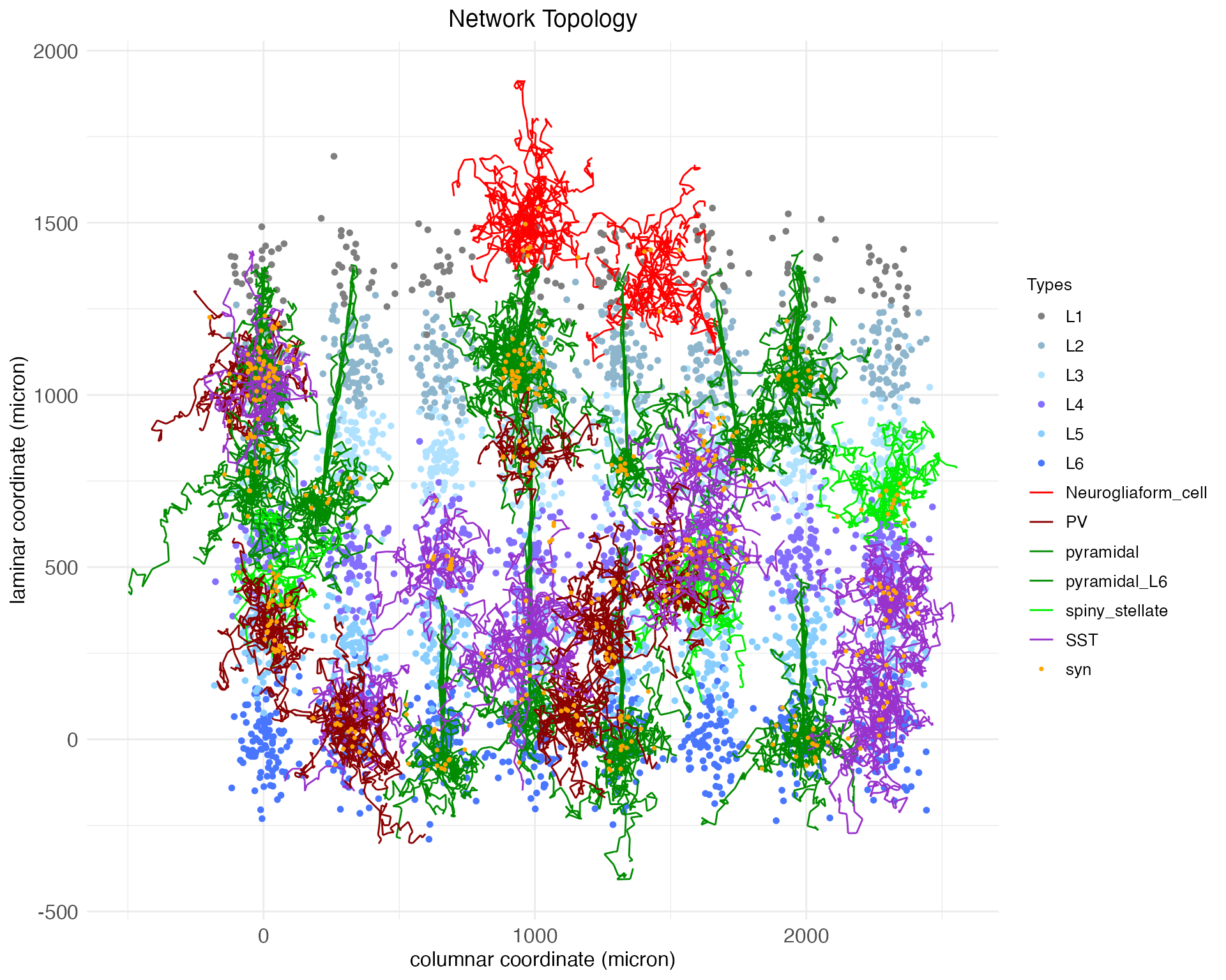
By default, the plot.network function plots all cell bodies as dots, colored by layer, and plots the arbors for a random 1% of those cell bodies, colored by cell type. Synapses are plotted as dots. The synapses shown are determined by the presynaptic axons that are plotted. Notice that the arbors shown are mostly small and compact, expect for the pyramidal neurons, which have long apical dendrites extending upwards. Notice also that the single subcortical layer, thalamus, is a further distance below the cortical layers than the cortical layers are below each other.
The plot gives coordinates in microns. Spatial coordinates giving a cell’s soma (i.e., body) location along the columnar (x), laminar (y), and patch-hemisphere (z) axes are continuous and real-valued. These coordinates are used in conjunction with soma-to-synapse distance (integrated along the axon) and a transmission velocity parameter to simulate spike propagation.
Seven parameters control the coordinates assigned to each network node: column diameter c_{\mathrm{diameter}}, layer height l_{\mathrm{height}}, column separation factor F_{\mathrm{column}}, layer separation factor F_{\mathrm{layer}}, patch separation factor F_{\mathrm{patch}}, subcortical separation factor F_{\mathrm{sub}}, and hemisphere separation factor F_{\mathrm{hemi}}. A node is created for each combination of zero-based integer-indexed patch p, layer l, column c, and hemisphere h. Each node is assigned a coordinate \langle x_c,y_l,z_{p\times h}\rangle: z_{p\times h} = p \frac{c_{\mathrm{diameter}}F_{\mathrm{patch}}}{2} + h \frac{c_{\mathrm{diameter}}F_{\mathrm{hemi}}}{2} y_l = l \frac{l_{\mathrm{height}}F_{\mathrm{layer}}}{2} x_c = c \frac{c_{\mathrm{diameter}}F_{\mathrm{column}}}{2} Cortical and subcortical layers are indexed by independent series l. The above formula for y_l is used in both cases; however, if computing node coordinates for subcortical layers, an addition term l_{\mathrm{height}}F_{\mathrm{sub}}/2 is subtracted from y_l. Within each node, a coordinate \langle z_n,y_n,x_n\rangle is assigned to each neuron n by sampling from a normal distribution: z_n \sim \mathcal{N}(z_{p\times h}, \frac{c_{\mathrm{diameter}}}{2}) y_n \sim \mathcal{N}(y_l, \frac{l_{\mathrm{height}}}{2}) x_n \sim \mathcal{N}(x_c, \frac{c_{\mathrm{diameter}}}{2}) By default, DACx sets c_{\mathrm{diameter}} = 120.0, l_{\mathrm{height}} = 180.0, F_{\mathrm{patch}} = 2.5, F_{\mathrm{column}} = 2.5, F_{\mathrm{layer}} = 2.5, F_{\mathrm{sub}} = 20, and F_{\mathrm{hemi}} = 40. The above network ACx_mini used larger values for the column and patch separation factors so that the columns would be more visually distinct in plots.
These default values were obtained via back-of-the-envelope calculations from widefield microscopy images of wild-type mouse auditory cortex. They can be extended to estimate values needed to simulate a complete brain area. By eyeballing those same images (multiplying pixels by a resolution of 0.4 microns per pixel), we estimate a mean neuronal soma diameter of 14 microns, cluster radius of 62 microns, and cluster density (i.e., proportion of cluster occupied by neuronal somas) of 0.4. These numbers imply approximately 278 cells per cluster. Assuming a span of 13 columns across the tonotopic axis of the auditory cortex (approximately 2 mm) and a patch depth of 3 perpendicular to it (approximately 0.5 mm), six layers at that cluster density is approximately 65,000 neurons total, which is a fair approximation for a single hemisphere of mouse auditory cortex. Of course, for demonstration purposes we will stick to the much smaller network we’ve already created, but these calculations show how the parameters of the set.network.structure function can be used to scale up to a more realistic network size.
Returning to our demonstration network, we have only “local” connections between neighboring neurons. Next, we will add meso-scale and long-range connections using circuit motifs.
Circuit motifs
A circuit motif, represented in the DACx package by special objects of class motif, is a predefined pattern of connections between layers and columns in a network, either within a single cortical region or across regions. It is a recipe for directing axons – and thereby connecting cells – between nodes, based on (1) cell type and (2) pre and post-synaptic node coordinates.6
Below we will define and load six canonical circuit motifs thought to characterize sensory cortex:
- Principal columnar projections: a translaminar and intracolumnar projection motif of principal (i.e., excitatory) columnar projections (Harris and Mrsic-Flogel 2013).
- Auditory lateral projections: a lateral projection motif for cross-columnar communication (Park and Geffen 2020).
- Bottom-up intracolumnar inhibitory projections: a translaminar deep-layer PV arborization motif for intracolumnar inhibition (Bortone et al. 2014, Frandolig et al. 2019).
- Top-down intracolumnar inhibitory projections: a motif for intracolumnar inhibition based around the neurogliaform cells of L1 and the apical dendrites of pyramidal neurons (Huang et al. 2024).
- Thalmacortical projections: from the thalamus up into the cortex, providing the cortex with sensory input from the periphery.
- Corpus callosum: Projections connecting the cortex of the two hemispheres (Barbaresi et al. 2024).
Roughly speaking, these motifs are “columnar”, in the sense that they are defined relative to a single cortical column and repeated across all columns, both along the primary columnar axis sized by n_columns and the secondary columnar axis sized by n_patches.
Principal columnar projections
The new.motif function initializes an empty motif object. Let’s initialize one to model the canonical translaminar, intracolumnar principal (i.e., excitatory) projections in the sensory cortex. These connections are largely what defines a “column” in the cortex, and thus they connect neurons in different layers while staying within the same column.
motif.pp <- new.motif(motif_name = "principal projections")Connections between layers are added to the motif using the load.projection.into.motif function. This function takes as arguments the motif object, the source layer name, and the target layer. By default, it extends the axons of principal cells in the source layer to principal cells in the target layer with a connection strength of 0.1 nS (equivalent to a 5 pA current at 50 mV). The connection strength value, held in the variable connection_strength, is used to control the expected initial strength of synapses along the extended axon. This value can be modified via a fourth argument to the function. Here, for example, we load projections with connection strength of 0.2 nS from layer L4 to layer L2 and layer L3 into our new motif:
motif.pp <- load.projection.into.motif(motif.pp, "L4", "L2", 0.2)
motif.pp <- load.projection.into.motif(motif.pp, "L4", "L3", 0.2)We have increased the strength of this connection from the default because layer 4 (the primary site of input from outside the cortex into the cortex) has its strongest intra-cortical projections to layers 2 and 3. By default, the loaded projections are between principal neurons, which for layer 4 are spiny stellate cells and for layers 2 and 3 are pyramidal neurons. Below we will show how the pre and post-synaptic cell types can be modified through additional function arguments. For now, let’s load weaker projections from layer 4 into the deep layers below it:
motif.pp <- load.projection.into.motif(motif.pp, "L4", "L5", 0.05)
motif.pp <- load.projection.into.motif(motif.pp, "L4", "L6", 0.05)The column-defining principle projections also typically include recurrent loops between layers 2 and 3 and layer 5, which we’ll assume are of average (i.e., default) strength:
motif.pp <- load.projection.into.motif(motif.pp, "L2", "L5")
motif.pp <- load.projection.into.motif(motif.pp, "L3", "L5")
motif.pp <- load.projection.into.motif(motif.pp, "L5", "L2")
motif.pp <- load.projection.into.motif(motif.pp, "L5", "L3")Finally, these projections also include a feed-forward projection from layer 5 to layer 6, and a feedback projection from layer 6 to layer 4:
motif.pp <- load.projection.into.motif(motif.pp, "L5", "L6", 0.05)
motif.pp <- load.projection.into.motif(motif.pp, "L6", "L4", 0.05)With the complete principle-projection motif defined, we apply it using the apply.circuit.motif function. This function takes as arguments the network object and the motif object. It adds the connections defined in the motif to the network.
ACx_mini <- apply.circuit.motif(
ACx_mini,
motif.pp
)Let’s plot the results of applying this motif. We could update our original plot, i.e., plot the same cells arbors again, seeing how this motif has changed and grown them. The plot.network function returns not only the generated plot, but also the indexes for the plotted somas (in soma_mask) and arbors (in arbor_idx). This allows for plots to be reproduced as a network is built out, showing the same cell arbors as more motifs are added.
However, as the emphasis here is the motif itself, we will instead use the plot_motif to specify that we want to plot arbors which were in part built from a specific motif. Cell arbors are potentially the result of multiple motifs, e.g., local connections plus principal projections plus anything else we add. By specifying “principal projections”, the entire arbor cell each randomly selected cell (by default, 1% of available cells) will be plotted, not just the portion of the arbor constructed from the principal projections motif. Still, we get a sense for the shape of the motif and how it connects cells in the network.
plt <- plot.network(
ACx_mini,
plot_motif = "principal projections"
)
plt$plot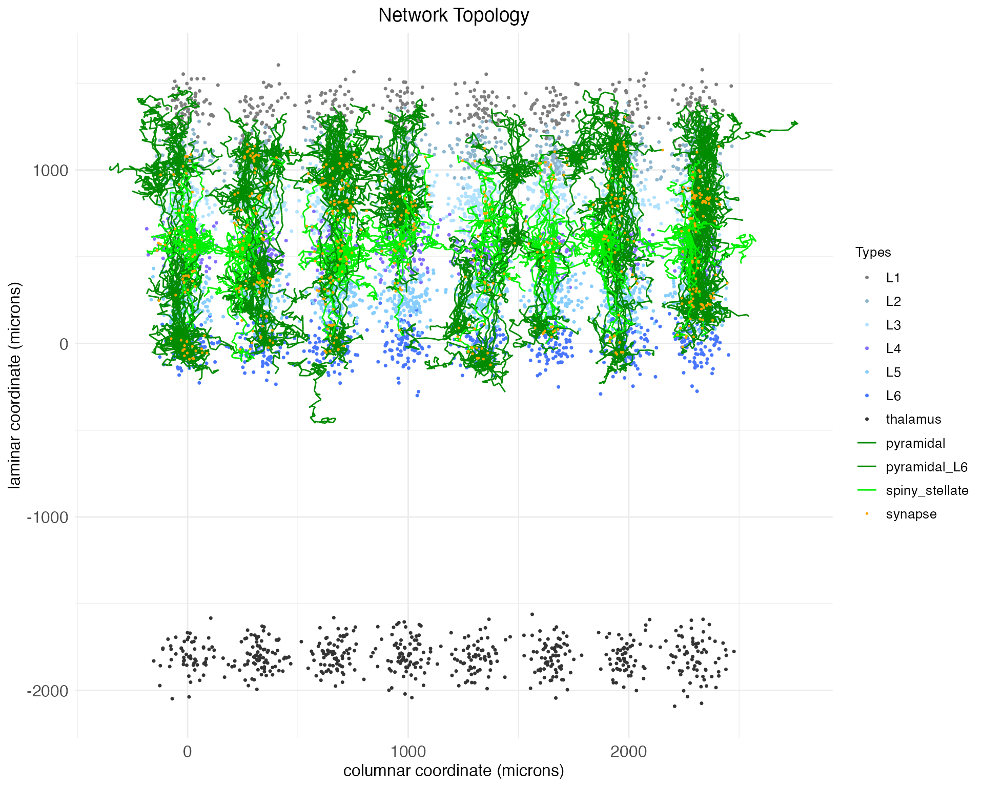
We can also plot the network in 3D, showing the full spatial shape of the arbors. To ensure we are plotting the same arbors shown in the 2D plot above, this time we will use the arbor_idx argument and the previously returned arbor indexes.
plt <- plot.network(
ACx_mini,
arbor_idx = plt$arbor_idx,
threedim = TRUE,
plot_motif = "principal projections"
)
plt$plotNotice, as is clear in both the 2D and 3D plots, that while the arbors cross between layers, they all mostly remain in column. There are no meso-scale lateral projections between columns.
Auditory lateral projections
Within sensory cortex, cortical columns tend to respond to a single type of stimulus. For example, cortical columns in the visual cortex might have preferred edge orientations while columns in the auditory cortex prefer certain sound frequencies. More advanced cortical computations require integrating input from a range of stimuli (e.g., a range of edge orientations or sound frequencies), and thus there must be some mechanism of column cross-talk. This is thought to be accomplished by lateral connections between cells of the same layer, but different columns. For example, Park and Geffen (2020) propose that these lateral connections include (1) excitatory projections from principal cells out to principal cells and PV and SST interneurons in adjacent columns and (2) inhibitory projections from SST interneurons out specifically to principle (excitatory) neurons in adjacent columns. Thus, for this motif, we need to make use of the presynaptic_type and postsynaptic_type arguments of the load.projection.into.motif function to specify the relevant neuron types for each projection.
By default, load.projection.into.motif creates projections within the same column. To create lateral projections, we need to use the max_col_shift_up and max_col_shift_down arguments of the function to specify how many columns away from the source column the target column can be. For the purposes of this demonstration, we’ll set these to four. However, lateral projections are assumed to drop off exponentially, and so when the apply.circuit.motif function is called, the actual length of any lateral branch projection will be a random value placing its expected endpoint somewhere between the source column and four columns away.
The arguments max_pch_shift_up and max_pch_shift_down serve the same function for spreading lateral projections along the secondary columnar axis. In this case, we’ll set the values to the patch axis to two. When lateral projections are expected along both columnar axes, they grow as some random linear combination of one of the following four (randomly choosen) cardinal direction pairs: {column-up, patch-up}, {column-down, patch-down}, {column-up, patch-down}, and {column-down, patch-up}. The same exponential decay applies.
motif.ACxlat <- new.motif(motif_name = "ACx laterals")
# Add projection for each layer
for (layer in c("L2", "L3", "L4", "L5", "L6")) {
# Excitatory laterals
for (celltype in c("principal", "PV", "SST")) {
motif.ACxlat <- load.projection.into.motif(
motif.ACxlat,
presynaptic_layer = layer,
postsynaptic_layer = layer,
presynaptic_type = "principal",
postsynaptic_type = celltype,
max_col_shift_up = 4,
max_col_shift_down = 4,
max_pch_shift_up = 2,
max_pch_shift_down = 2
)
}
# Inhibitory laterals
motif.ACxlat <- load.projection.into.motif(
motif.ACxlat,
presynaptic_layer = layer,
postsynaptic_layer = layer,
presynaptic_type = "SST",
postsynaptic_type = "principal",
max_col_shift_up = 4,
max_col_shift_down = 4,
max_pch_shift_up = 2,
max_pch_shift_down = 2
)
}As before, we can apply this motif and visualize the results:
ACx_mini <- apply.circuit.motif(
ACx_mini,
motif.ACxlat
)
plt <- plot.network(
ACx_mini,
threedim = TRUE,
plot_motif = "ACx laterals"
)
plt$plotNow we have not only vertical projections between layers, but horizontal projections between columns.
Bottom-up intracolumnar inhibitory projections
Cortical computations require careful balance between excitatory and inhibitory activity, both within local nodes and between nodes within columns. Balancing the principal columnar projections – which are predominantly excitatory – are two types of inhibitory projections. The first are intracolumnar inhibitory projections from PV interneurons out of L6 (Bortone et al. 2014, Frandolig et al. 2019). These function to shut the column down and are largely driven by bottom-up thalamic input.
Let’s define a motif for these inhibitory projections. For this motif, we again need to make use of the presynaptic_type and postsynaptic_type arguments of the load.projection.into.motif function to specify that this projection motif is from inhibitory PV neurons to excitatory principal neurons.
motif.Binhib <- new.motif(motif_name = "bottom-up inhibition")
motif.Binhib <- load.projection.into.motif(
motif.Binhib,
presynaptic_layer = "L6",
postsynaptic_layer = c("L5", "L4", "L3", "L2"),
presynaptic_type = "PV",
postsynaptic_type = "principal"
)For now, we will define only the PV \rightarrow principal component of this motif. The fact that the PV cells themselves receive input from the thalamus will be handled later, via the thalamic input motif. As before, we can apply this motif and visualize the results.
ACx_mini <- apply.circuit.motif(
ACx_mini,
motif.Binhib
)
plt <- plot.network(
ACx_mini,
threedim = TRUE,
plot_motif = "bottom-up inhibition"
)
plt$plotAs can be seen, now the deep-layer PV cell arbors (in magenta) are extending their axons upwards towards the superficial layers, as expected from the motif.
Notice that in this case we’ve loaded multiple projections at once by specifying a vector of target layers. While the argument presynaptic_layer can take only a single value, if postsynaptic_layer is given a vector of layer names, projections will be loaded from the presynaptic layer to each of the specified postsynaptic layers. In this case, the pre and post-synaptic neuron types are the same for each projection, but if different types were required, then multiple calls to the load.projection.into.motif function would be necessary.
Top-down intracolumnar inhibitory projections
The second type of inhibitory projections balancing excitatory input are driven by neurogliaform cells in L1. Within the cortex, L1 is distinct insofar as it consists almost entirely of the tufts of apical dendrites from lower-layer pyramidal cells. Roughly speaking (and consistent with how DACx implements circuit topologies), cortical pyramidal cells receive local and meso-scale input on their basal dendrites, while large apical dendrites receive “top-down” feedback from higher cortical areas (e.g., apical dendrites from V1 receive input from V2) and higher-order thalamus.
While DACx does not support multiple cortical regions within a single hemisphere (e.g., a V2 functionally distinct from V1),7 it does support modeling a second circuit pattern involving apical dendrites. The apical dendrites of pyramidal cells receive inhibitory input from the neurogliaform cells in L1 (Huang et al. 2024). To implement this motif in DACx, we use the via_apical argument while keeping presynaptic and postsynaptic layers the same.
motif.Tinhib <- new.motif(motif_name = "top-down inhibition")
# neurogliaform targeting of apical dendrites
motif.Tinhib <- load.projection.into.motif(
motif.Tinhib,
presynaptic_layer = "L1",
postsynaptic_layer = "L1",
presynaptic_type = "neurogliaform_cell", # "principal" would work too
postsynaptic_type = "pyramidal",
via_apical = TRUE
)Neurogliaform cells also target each other and nearby L2/3 PV interneurons.
# neurogliaform self-targeting
motif.Tinhib <- load.projection.into.motif(
motif.Tinhib,
presynaptic_layer = "L1",
postsynaptic_layer = "L1",
presynaptic_type = "neurogliaform_cell",
postsynaptic_type = "neurogliaform_cell"
)
# neurogliaform PV-targeting
motif.Tinhib <- load.projection.into.motif(
motif.Tinhib,
presynaptic_layer = "L1",
postsynaptic_layer = c("L2", "L3"),
presynaptic_type = "neurogliaform_cell",
postsynaptic_type = "PV"
)SST interneurons in L2/3 complete this meso-scale inhibitory circuit by targeting both the L1 neurogliaform cells and the L1 apical tufts of L2/3 pyramidal cells. However, as we’ve set the network up so far, we are not able to implement this projection. We could set via_apical to TRUE and set postsynaptic_layer to c(“L2”, “L3”), but this would not work. The effect of setting via_apical to TRUE is to find synapses only along apical dendrites and to determine which cells to check by whether they have an apical dendrite targeting the postsynaptic layer instead of by whether their soma is located in the postsynpatic layer.
In line with how the biology itself works, implementing this projection in DACx would require distinguishing L2/3 pyramidal cells from other kinds of pyramidal cells. We would then set postsynaptic_layer to L1, so that axons went to the location of the apical dendrites, and set postsynaptic_type to this new L2/3-specific pyramidal cells, so that these axons only synapsed with the apical dendrites of pyramidal cells in L2/3. These changes would be relatively straightforward, but we will not implement them in this tutorial.
What about the sources of input to neurogliaform cells? These cells receive input from non-local sources, such as higher order cortex and thalamus, but also from L5 IT pyramidal and L6b pyramidal cells.8 While we haven’t set up a special cell type for L5 IT pyramidal cells or distinct types of L6 pyramidal cells, for demonstration purposes we can use the pyramidal_L6 as a stand in:
# Local columnar input
motif.Tinhib <- load.projection.into.motif(
motif.Tinhib,
presynaptic_layer = "L6",
postsynaptic_layer = "L1",
presynaptic_type = "pyramidal_L6",
postsynaptic_type = "neurogliaform_cell"
)Let’s finally apply and view the motif:
ACx_mini <- apply.circuit.motif(
ACx_mini,
motif.Tinhib
)
plt <- plot.network(
ACx_mini,
threedim = TRUE,
plot_motif = "top-down inhibition"
)
plt$plotThalmacortical projections
Thus far we’ve only created meso-scale connections within a single cortical region. However, we also need connections between regions. First, we need our subcortical region (the thalamus) to talk to the cortical region above it. The thalamus receives its inputs from the periphery. In the case of audition, this means the cochlea. Thalmacortical cells in the auditory thalamus send their inputs to the auditory cortex in a way which preserves the tonotopic axis of auditory processing. For simplicity, we will assume that tonotopy is preserved because projections stay in column, without lateral shifts. Further, while thalmacortical projections synpase into all cortical layers (except L1), the connections to L4 are the strongest.
The thalmacortical projection motif is implemented as follows:
motif.tc <- new.motif(motif_name = "thalmacortical projections")
motif.tc <- load.projection.into.motif(motif.tc, "thalamus", "L4", 0.2)
motif.tc <- load.projection.into.motif(motif.tc, "thalamus", "L2", 0.05)
motif.tc <- load.projection.into.motif(motif.tc, "thalamus", "L3", 0.05)
motif.tc <- load.projection.into.motif(motif.tc, "thalamus", "L5", 0.05)
motif.tc <- load.projection.into.motif(motif.tc, "thalamus", "L6", 0.05)The above projections all involve principal thalamic cells synapsing onto principal cortical cells. However, there is some evidence that the thalmacortical projections into L6 also target the same PV cells involved in the intracolumnar inhibitory motif (Frandolig et al. 2019), with stronger input than received by the principal excitatory cells.
motif.tc <- load.projection.into.motif(
motif.tc,
presynaptic_layer = "thalamus",
postsynaptic_layer = "L6",
postsynaptic_type = "PV"
)Let’s apply and plot it:
ACx_mini <- apply.circuit.motif(
ACx_mini,
motif.tc
)
plt <- plot.network(
ACx_mini,
threedim = TRUE,
plot_motif = "thalmacortical projections"
)
plt$plotCorpus callosum
The second type of inter-region connection that’s needed is between the cortices of the two hemispheres. In mammals, this is largely accomplished by the corpus callosum. While the exact nature of the corpus callosum varies by species and is disputed, we will assume that callosal projections preserve layer and column identity, connect the hemispheres only at L3 and L5, and include both excitatory cells (callosal pyramidal neurons) and inhibitory cells (callosal PV interneurons).
Let’s build and apply the corpus callosum motif. As can be seen in the code, the key is the hem_shift argument. Here we have set it to 1, which means that the postsynaptic layer and column are located in the contralateral hemisphere. The default value of hem_shift, used above in all other motif projections, is 0. This default keeps the postsynaptic layer and column within the same hemisphere as the presynaptic layer and column.
motif.CC <- new.motif(motif_name = "corpus callosum")
motif.CC <- load.projection.into.motif(motif.CC, "L3", "L3", presynaptic_type = "callosal_pyramidal", postsynaptic_type = "pyramidal", hem_shift = 1)
motif.CC <- load.projection.into.motif(motif.CC, "L5", "L5", presynaptic_type = "callosal_pyramidal", postsynaptic_type = "pyramidal", hem_shift = 1)
motif.CC <- load.projection.into.motif(motif.CC, "L3", "L3", presynaptic_type = "callosal_PV", postsynaptic_type = "pyramidal", hem_shift = 1)
motif.CC <- load.projection.into.motif(motif.CC, "L5", "L5", presynaptic_type = "callosal_PV", postsynaptic_type = "pyramidal", hem_shift = 1)
ACx_mini <- apply.circuit.motif(
ACx_mini,
motif.CC
)And update our plot:
plt <- plot.network(
ACx_mini,
threedim = TRUE,
plot_motif = "corpus callosum"
)
plt$plotNetwork topology summary
Let’s return again to the fetch.network.components function and look at the network now:
ACx_mini_comps <- fetch.network.components(ACx_mini, include_arbors = TRUE, return_arbors = FALSE)## Summary of network:
## Number of neurons: 5853
## Number of synapses: 51136
## Hemisphere names: left, right
## Number of hemispheres: 2
## Subortical layer names: thalamus
## Number of subcortical layers: 1
## Cortical layer names: L6, L5, L4, L3, L2, L1
## Number of cortical layers: 6
## Number of columns: 8
## Number of patches: 4
## Cell types used: pyramidal_L6, SST, VIP, PV, pyramidal, callosal_pyramidal, callosal_PV, spiny_stellate, neurogliaform_cell, thalmacortical
## Motifs used: local connections, principal projections, ACx laterals, bottom-up inhibition, top-down inhibition, thalmacortical projections, corpus callosumIn addition to what’s printed, the function also extracts other important summary information. For example, here are the mean numbers of synapses per pre-synaptic neuron, per cell type:
## neuron_type n_synapses
## 1 callosal_PV 10.820789
## 2 callosal_pyramidal 11.491049
## 3 neurogliaform_cell 6.311653
## 4 PV 7.240803
## 5 pyramidal 10.910382
## 6 pyramidal_L6 8.055363
## 7 spiny_stellate 8.209540
## 8 SST 7.751880
## 9 thalmacortical 3.868056
## 10 VIP 6.171171Before concluding, two other plotting options are helpful in exploring a network’s topology. First, for both 2D and 3D plots, the complex arbors can be replaced by straight-line edges between pre and post-synaptic cells, allowing synaptic connections to be seen directly. For example, we see only synaptic connections added as a result of applying the lateral projection motif:
plt_lat <- plot.network(
ACx_mini,
plot_motif = "ACx laterals",
reconstruct_arbors = FALSE
)
plt_lat$plot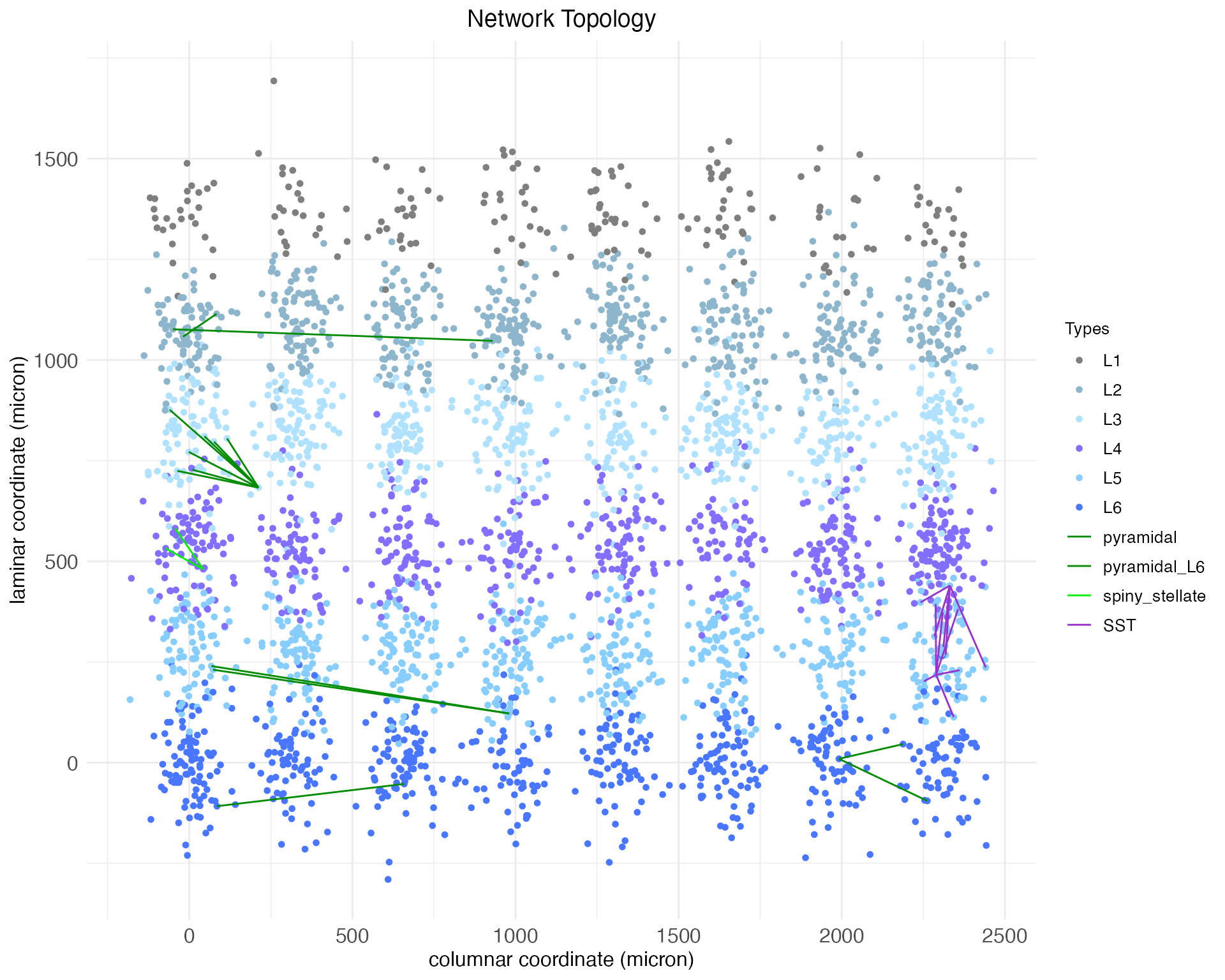
For both 2D and 3D plots, cell arbors can be colored by process type, i.e., whether they are an axon or dendrite. Here, for example, is our network plotted in 3D with a random 1% of arbors colored by process type:
plt <- plot.network(
ACx_mini,
threedim = TRUE,
edge_color = "is_axon"
)
plt$plotTo conclude, let’s plot 10% of process arbors (colored by cell type) to get a feel for the full richness of the network:
plt <- plot.network(
ACx_mini,
threedim = TRUE,
arbor_density = 0.1
)
plt$plot