Excitatory-inhibitory feedback loops
Michael Barkasi
August 16, 2026 (v1.1)
tutorial_EI_loops.Rmd
Introduction
The brain processes information in parallel. For example, when you watch an egg fall and hit the ground, the resulting splat both makes a sound and has an appearance. The sound is perceived through your ears and brought to consciousness through processing in one part of your brain, while the appearance is perceived through your eyes and brought to consciousness through a different part of your brain. It use to be thought that these distinct processing streams have to come together in a third part of your brain in order for you to have a unified auditory-visual experience of a splattering egg. Nowadays, it’s generally thought that the unification, or “binding”, happens instead by synchronizing activity across auditory and visual areas of the brain. That is, the spiking representing the appearance happens at the same time as the spiking representing the sound.
This synchronization happens at different frequencies, depending on the task. For a task such as perceptual binding, the synchronization is a “gamma wave”, i.e., an oscillation of overall network behavior in the range of 30-80 Hz. What is the mechanism of this gamma-wave synchronization? How is it that distant areas of the brain not only come to fire together, but fire together in specific frequency ranges?
For synchronized gamma waves, it’s generally thought that the work is done by the interaction of a few powerful fast-spiking inhibitory cells with larger populations of slower excitatory cells (Kim et al. 2015). These two cell types interact in recurrent loops within a single brain region to produce gamma-wave oscillations, with between-region inhibitory connections providing the between-region synchronization.
Excitatory-Inhibitory feedback loops are a general mechanism for producing oscillations. What is it about this particular combination of a few fast-spiking inhibitory cells and a larger population of slower excitatory cells which specifically produces gamma-wave frequencies? As a first step to answering this question, we can model the combination in a single network node with a biological growth-transform (BGT) simulation. This will allow us to (1) see that realistic network-scale gamma-wave activity emerges from the interaction of a specific combination of single-cell biological behavior and (2) verify that the BGT framework reproduces the expected network-scale activity from that specific combination.
Population parameters
Let’s set up our population of interacting excitatory and inhibitory cells. We begin by setting up the R environment: clearing the workspace, setting a random-number generator seed, and loading the DACx package.
# Clear the R workspace to start fresh
rm(list = ls())

# Set seed for reproducibility
set.seed(12345)

# Load DACx package
library(DACx, quietly = TRUE)
Next, we create a new network object with the new.network function.
network.node <- new.network()The object initialized by new.network is an empty shell for a single single-node network. For this tutorial, we will leave the network a single node. It will include two distinct neuron types: an excitatory type, based on layer 4 principal neurons (spiny stellates), and an inhibitory type, based on parvalbumin (PV) interneurons.
The choice of spiny stellates for the excitatory cells is different from the canonical excitatory-inhibitory cortical circuit thought to induce gamma-waves. Canonically, the circuit would be PV cells interacting with pyramidal neurons. However, for this demonstration we need only a generic slow-responding excitatory cell. The defining topological feature of pyramidal neurons – their large apical dendrites – would complicate the demonstration in unnecessary ways. Thus, we’ll use spiny stellates for our slow-responding excitatory cells.
Defining cell types
DACx comes with preloaded cell types and the function modify.cell.type, which is able to both modify existing cell types and add new ones based on existing ones. Although spiny stellate and PV cells come preloaded, we will set them up from scratch to ensure reproducibility.1
To start, let’s grab the generic “neuron” type and set all parameters to something reasonable. For full details about the meaning of these parameters, see the tutorials on cell types and the mathematics of biological growth-transform models.
modify.cell.type(
    old_type_name         = "neuron", # Type to use as base
    new_type_name         = NULL,     # If NULL, modify old type in place; else copy old type into new type with this name
    # Membrane kinetics
    tau_fast              = 2.5,   # ms
    tau_slow              = 60.0,  # ms
    tau_Vs                = 100.0, # ms/spike
    dCdr                  = 0.01,  # concentration/spike
    dVdr                  = 0.05,  # concentration/spike
    max_spike_rate        = 0.1,   # spikes/ms
    g_leak                = 5.0,   # nS
    # Intercell transmission
    spike_velocity        = 500,   # micons/ms, = 0.5 m/s
    spine_density         = 0.0,
    axon_target           = "dendrite_shaft",
    # Spiking
    I_spike               = 1e3,   # pA
    dHdv_bound            = 1.05,
    v_spike               = 35,    # mV
    tau_spike             = 1.0,   # ms
    v_threshold           = -55,   # mV
    v_eq                  = list ( # mV
      "spiny stellate" = 0.0,    # Excitatory, so drives postsynaptic cell membrane v up
      "PV"             = -80.0), # Inhibitory, so drives postsynaptic cell membrane v down
    # Membrane characteristics
    v_rest                = -70,   # mV
    v_bound               = 1.15,
    g_syn                 = list(  # nS
      "spiny stellate" = 0.1,
      "PV"             = 0.1),
    tau_syn               = list(  # ms
      "spiny stellate" = 2.0,   # Excitatory glutamate channels close quickly
      "PV"             = 6.0),  # Inhibitory GABA channels stay open longer
    # Neurite structure
    axon_branch_count     = 20,
    dendrite_branch_count = 20,
    branch_independence   = 0.75,
    branch_spread         = 0.75,
    apical_target_layer   = "none"
  )
To create our PV and spiny stellate cells, we will now copy our generic “neuron” type into two new cell types, with the appropriate modifications. PV interneurons are highly responsive cells with a high rate of fire, little adaptation (i.e., little short-term depression), and little memory – that is, they have a high leak current and so don’t integrate signals. Thus, they function as coincidence detectors (integrating only near-simultaneous input spikes) and send strong inhibitory signals.
modify.cell.type(
    old_type_name  = "neuron", # Type to use as base
    new_type_name  = "PV",     # If NULL, modify old type in place; else copy old type into new type with this name
    # Membrane kinetics
    tau_fast       = 1.0,    # ms, Short for fast responses
    tau_Vs         = 2.5,    # ms/spike, Fast recovery for little adaptation
    dVdr           = 0.025,  # concentration/spike, Low vesicle rate for fast spiking
    max_spike_rate = 0.5,    # spikes/ms, High max spike rate
    g_leak         = 10.0,   # nS, Hight leak conductance for fast kinetics
    # Spiking
    I_spike        = 2e3,    # pA, High-current spikes
    tau_spike      = 0.3,    # ms, Short-duration spikes
    v_threshold    = -50,    # mV, Slightly higher threshold
    spine_density  = 0.0,    # ineffectual as of v1.1, setting for later
    axon_target    = "soma", # ineffectual as of v1.1, setting for later
    # Set synaptic weights
    g_syn          = list(   # nS
      "spiny stellate" = 2.0,
      "PV"             = 1.0)
  )
Conversely, spiny stellate cells are slower to respond, have higher adaptation, but more memory. They serve as signal integrators, integrating input spikes over longer time stretches.
modify.cell.type(
    old_type_name  = "neuron",         # Type to use as base
    new_type_name  = "spiny stellate", # If NULL, modify old type in place; else copy old type into new type with this name
    # Membrane kinetics
    tau_fast       = 5.0,     # ms, Long for slow responses responses
    g_leak         = 1.0,     # nS, Low conductance for slow kinetics
    # Intercell transmission
    spike_velocity = 100,     # microns/ms, slower transmission than PV cells
    spine_density  = 0.5,     # ineffectual as of v1.1, setting for later
    axon_target    = "spine", # ineffectual as of v1.1, setting for later
    # Membrane characteristics
    g_syn          = list(  # nS
      "spiny stellate" = 0.4,
      "PV"             = 4.0)
  )
Notice that defining the cell types involves setting an argument g_syn, taking a list which each cell type as a named entry. This argument gives the conductance (in nS) of the cell type’s synapses, for each pre-synaptic cell type. So, the above settings imply that PV connections onto spiny stellates are 10x stronger (4.0nS) than connections from other spiny stellates (0.4nS). These values are not strictly faithful to the actual biology, they are not a gross misrepresentation and will be suitable for modeling a simple excitatory-inhibitory feedback system with no other cell types.
Set network structure
Mimicking the structure of the brain, nodes are arrayed into layers and columns, cortical and subcortical regions, and hemispheres. This structure is set with the set.network.structure function. As we want to leave our network a single node, we leave out arguments related to this structure. However, the set.network.structure also controls the expected count for each node. We will use it to set an expected count of 50 for the spiny stellates and 5 for the PV interneurons.
n_ss <- 50
n_PV <- 5
sn   <- 20
network.node <- set.network.structure(
    network.node,
    neuron_types          = c("spiny stellate", "PV"),
    neurons_per_node      = c(n_ss, n_PV),
    synaptic_neighborhood = sn # microns
  )
By default, the set.network.structure function initializes local recurrent connections within each created node (in this case, a single node). The node we just created can be visualized with the plot.network function. To keep the plot clean, we can use the arbor_density argument, which controls the proportion of cells for which the generated arbors are shown.
plt <- plot.network(network.node, arbor_density = 0.1)
plt$plot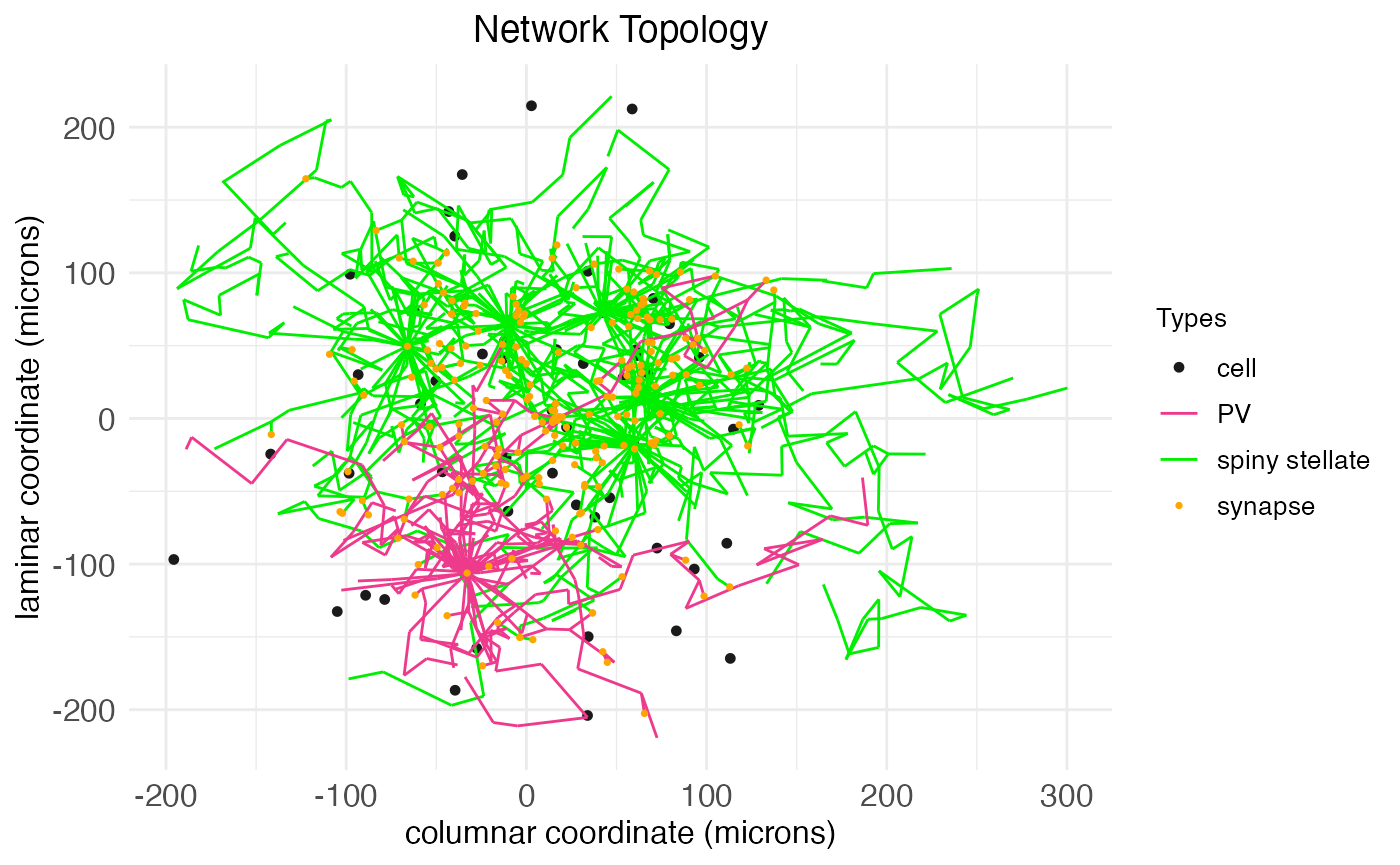
The arbors are generated via a biased random walk, the biasing factors fixed by cell type. The arbors include both axons and dendrites, which can be visualized explicitly by changing the arbor coloring. Although cells and arbors to-be-plotted are selected randomly, the plot.network function returns masks for the cells and arbors plotted, and can take this information to re-plot the same data again under different settings, e.g., coloring by arbor type instead of by cell type:
plt <- plot.network(
    network.node,
    arbor_density = 0.1,
    soma_mask     = plt$soma_mask,
    arbor_idx     = plt$arbor_idx,
    edge_color    = "is_axon"
  )
plt$plot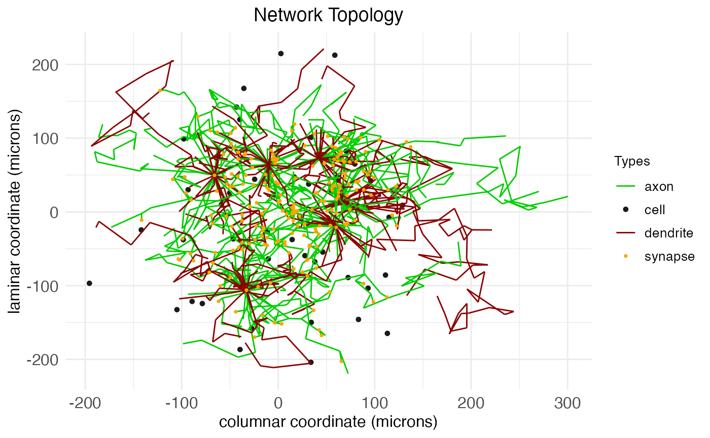
Examining network connectivity
The existence and number of connections between cells – synapses, colored orange in the above plots – are determined by the proximity of axons to dendrites. After the arbors are created, a separate algorithm looks for axon nodes within a certain small neighborhood (set by synaptic_neighborhood) of dendrite nodes and, if one is found, extends the axon to connect with the dendrite.
As the axis labels indicate, BGT models assign to each neuron a spatial coordinate giving its location along the laminar, columnar, and patch axes.2 All coordinates are continuous and real-valued and are used in conjunction with the spike velocity parameter to simulate spike propagation over the axonal arbors. While the above are 2D plots (which drop the patch axis), we can plot a 3D representation of our node, colored by cell type:
plt <- plot.network(
    network.node,
    arbor_density = 1.0,
    soma_mask     = plt$soma_mask,
    arbor_idx     = plt$arbor_idx,
    threedim      = TRUE
  )
plt$plot
As can be seen, even for a small single node, the arborization and number of synapses can be extensive. We can quantify the extent by calling the fetch.network.components function, which returns a list of all components of the network, including a print out of summary data:
ntw <- fetch.network.components(network.node, include_arbors = TRUE)## Summary of network:
## Number of neurons: 55
## Number of synapses: 1655
## Hemisphere names: left
## Number of hemispheres: 1
## Subortical layer names:
## Number of subcortical layers: 0
## Cortical layer names: layer
## Number of cortical layers: 1
## Number of columns: 1
## Number of patches: 1
## Cell types used: spiny stellate, PV
## Motifs used: local connectionsAll of the above plots show the spatially extended arbors which produce synaptic connections between cells. If we want to visualize just the connections without the mess of the arbors, we can do so by setting reconstruct_arbors to FALSE. This represents connections between cells in the familiar form of straight edges. By plotting all arbors, we see that our network is more-or-less fully connected.
plot.network(
    network.node,
    arbor_density      = 1.0,
    reconstruct_arbors = FALSE
  )$plot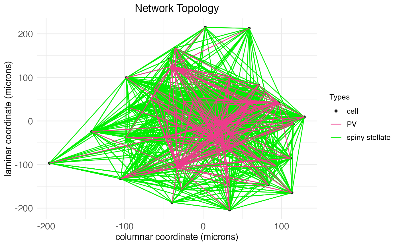
Simulating gamma waves
With our population of slow-responding excitatory (spiny stellate) and fast-responding inhibitory (PV) cells wired up, all that’s left is to run the simulation. While some tweaking of synaptic conductance (g_syn) is expected to ensure the feedback cycle is balanced, if a BGT simulation can reproduce the natural emergence of gamma waves in this population, it should do so more-or-less “out of the box”, without excessive tweaking of the parameters related to cell responsiveness.
Simulation parameters
The function run.BGT runs a simulation of spiking activity across a network using a BGT model. The function is just a wrapper over the BGT method of C++ network objects. It takes four arguments:
- network: A network created by the new.network function and structured by the set.network.structure function.
- I_stim: A matrix of input currents (in pA) over the duration of the simulation, rows representing neurons and columns representing time bins.
- dt: Time-step size for simulation, in ms. Default is 10^{-3}.
- initial_potential: Initial value for membrane potential, applied to all cells. Default is -70 mV.
The number of columns of I_stim determines the length of the simulation. In essence, the function run.BGT answers the question: How would the network respond to this stimulus current over this amount of time?
We’ll run a 1,200 ms simulation for the node we created above. From the above call to fetch.network.components, we know there are 55 neurons in our network. We can load this value directly from the function output:
n_neurons <- ntw$n_neuronsThis gives us the number of rows needed in our stimulus current matrix. For the number of columns, we need to know the number of time steps required:
stim_time_ms <- 1200
dt           <- 1e-3
n_steps      <- stim_time_ms/dt
cat("Number of time steps in the simulation:", n_steps)
## Number of time steps in the simulation: 1200000Now, to induce any spiking at all, current needs to be injected into the network. (Within the energy minimization framework of BGT, spiking happens because it is less costly to reset to rest potential through a spike than to hold rest potential via active ion pumping.) If we inject current into both the excitatory and inhibitory cells, we risk overpowering the intrinsic membrane dynamics of the cells and externally pinning their behavior to a constant spiking rate. To induce the natural oscillation of the system, the trick is to inject the excitatory cells with just enough current to get them spiking, but not so much current that feedback from their own spiking and the induced spiking of the inhibitory cells is overpowered.
Ignition current
Let’s analytically estimate the needed current. We set the synaptic conductance of spiny stellates into themselves at g_{\mathrm{syn}}^{\mathrm{ss}\rightarrow\mathrm{ss}}=0.4 nS. Let’s assume that on average that our spiny stellates have a membrane potential of v=-60 mV when receiving a spike. Excitatory input has an equilibrium potential of v_{\mathrm{eq}}=0 mV, so the excitatory drive potential is expected to be v_{\mathrm{drive}}=v_{\mathrm{eq}}-v=60 mV. Hence, synaptic current is I_{\mathrm{syn}}=v_{\mathrm{drive}}g_{\mathrm{syn}}^{\mathrm{ss}\rightarrow\mathrm{ss}}=60.0 \times 0.4 = 24 pA. The leak conductance is g_{\mathrm{leak}}=1.0 nS. The leak potential is expected to be v_{\mathrm{leak}}=v-v_{\mathrm{rest}}=10.0 mV, for a I_{\mathrm{leak}}=v_{\mathrm{leak}}g_{\mathrm{leak}}=10.0\times 1.0=10.0 pA leak current. Each spiny stellate cell has N^{\mathrm{ss}\rightarrow\mathrm{ss}}=26 pre-synaptic spiny stellate partners. These cells have a spike width of \tau_{\mathrm{spike}}=1.0 ms with a post-spike exponential decay of \mathrm{exp}(-t/\tau_{\mathrm{spike}}) for \tau_{\mathrm{spike}}=2.0 ms, so (assuming a constant firing rate across the population) we can approximate the ratio of time r^\prime each spiny stellate is spiking as r^\prime=\frac{r(\tau_{\mathrm{spike}}+\int_{0}^{\infty} \mathrm{exp}(-t/\tau_{\mathrm{spike}})\,dt)}{1000.0}=\frac{r(1.0+2.0)}{1000.0}=0.003r for r the mean firing rate for cells in the population. Thus, the expected ratio of spiny stellates spiking at any one time is N_{\mathrm{ss}}r^\prime. Hence I_{\mathrm{syn total}}^+=I_{\mathrm{syn}}\frac{N^{\mathrm{ss}\rightarrow\mathrm{ss}}}{N_{\mathrm{ss}}}N_{\mathrm{ss}}r^\prime=I_{\mathrm{syn}}N^{\mathrm{ss}\rightarrow\mathrm{ss}}r^\prime=24 \times 26 \times r^\prime= 1.872 r is the expected total synaptic current at any one moment any one moment.
df <- data.frame(x = 0:100)
df$y <- 1.872 * df$x

ggplot2::ggplot(df, ggplot2::aes(x, y)) +
  ggplot2::geom_line() +
  ggplot2::labs(y = "Expected excitatory synaptic current (pA)", x = "Expected firing rate (Hz)") +
  ggplot2::theme_minimal()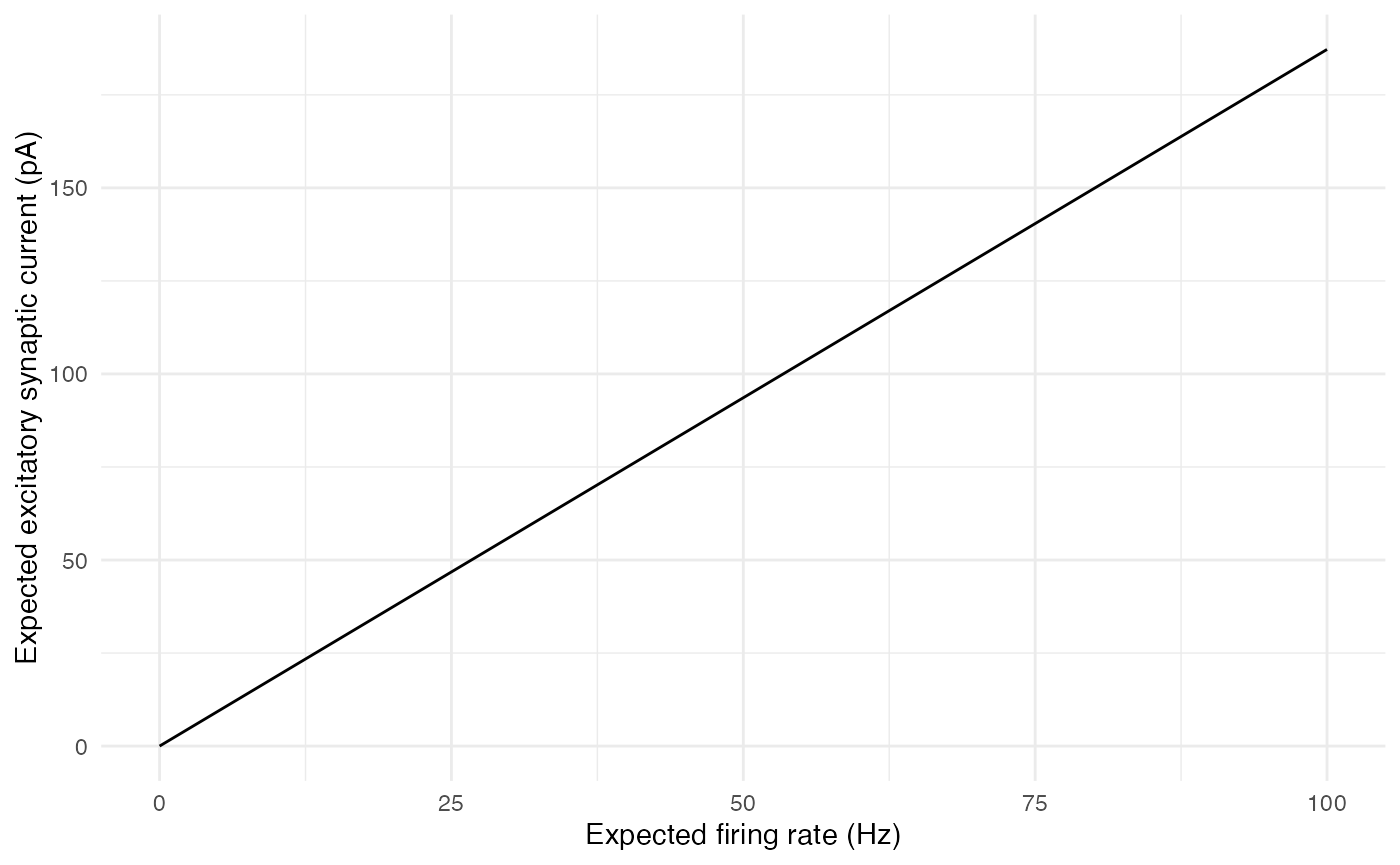
transfer <- function() {
  # Set up single unconnected spiny stellate cell
  net <- new.network()
  net <- set.network.structure(
    net,
    neuron_types     = "spiny stellate",
    neurons_per_node = 1
  )

  # Create sweep of 1 sec input currents
  dt          <- 1e-3          # ms per step
  n_steps     <- 1000 / dt     # 1000 ms = 1 second
  currents_pA <- seq(0, 300, by = 20)

  # Run simulations
  spike_rates_Hz <- vapply(currents_pA, function(I) {
    I_stim <- matrix(I, nrow = 1, ncol = n_steps)
    res    <- run.BGT(net, I_stim, dt)
    res$spike_counts[1]          # 1-s simulation of spike count == Hz
  }, numeric(1))

  # Plot results
  df <- data.frame(
      input_current_pA = currents_pA,
      spike_rate_Hz = spike_rates_Hz
    )
  ggplot2::ggplot(df, ggplot2::aes(input_current_pA, spike_rate_Hz)) +
    ggplot2::geom_line() +
    ggplot2::labs(
      title = "Empirical Estimate of Transfer Function",
      y     = "Spike rate response (Hz)",
      x     = "Input current (pA)"
    ) +
    ggplot2::theme_minimal()
}
transfer()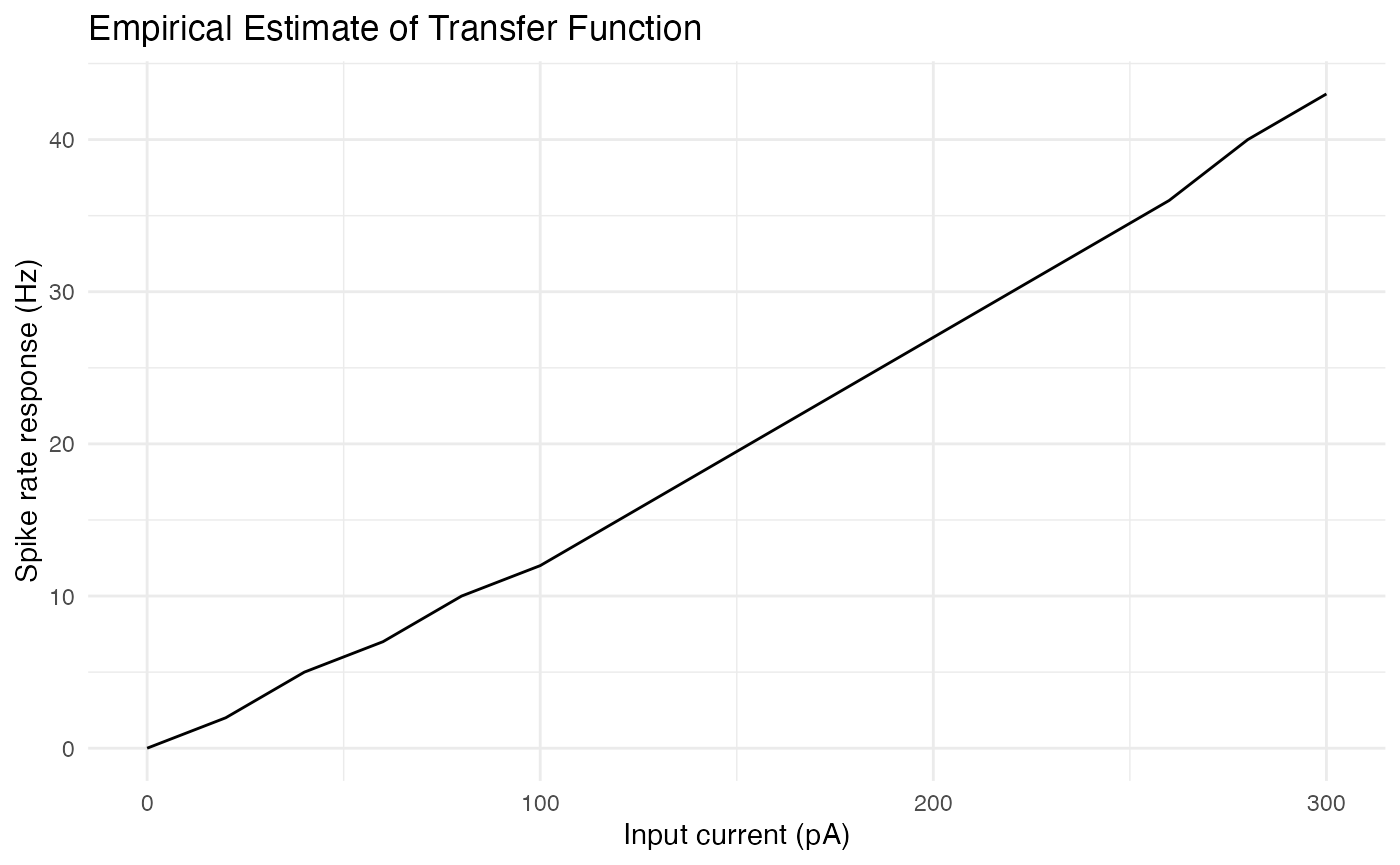
# Get edge list for local connections (pre/post neuron indices)
edges <- as.data.frame(ntw$edge_idx_by_type[1])
types <- ntw$neuron_type_name

# Annotate each edge with pre- and post-synaptic cell types
edges$pre_type  <- types[edges$pre_neuron_idx]
edges$post_type <- types[edges$post_neuron_idx]

# Count cells of each type (denominator for per-cell mean)
n_per_type <- table(types)

# Summarise: total connections and mean connections per pre-synaptic cell
edges |>
  dplyr::count(pre_type, post_type, name = "total_connections") |>
  dplyr::mutate(
    n_pre_cells      = as.integer(n_per_type[pre_type]),
    mean_connections = total_connections / n_pre_cells
  )
## pre_type post_type total_connections n_pre_cells mean_connections
## 1 PV PV 26 6 4.333333
## 2 PV spiny stellate 186 6 31.000000
## 3 spiny stellate PV 182 49 3.714286
## 4 spiny stellate spiny stellate 1261 49 25.734694To achieve this balance of “igniting” the feedback loop without overpowering it, we’ll use a constant 100 pA current. 1000 ms input current to just the spiny stellates, starting at 100 ms. We can compute the initial and final time steps of this current, plus a mask for the spiny stellates, as follows:
# Set stimulus start and length
stim_length_ms      <- 1000
stim_start_ms       <- 100
# Find start and end steps of the input stimulus current
stim_length         <- stim_length_ms / dt
stim_start          <- stim_start_ms / dt
stim_end            <- stim_start + stim_length - 1
# Find mask for principal neurons
spiny_stellate_mask <- ntw$neuron_type_name == "spiny stellate"
A final question is how much current to apply. For this simulation, we’ll use a constant current of 100 pA to the spiny stellates during the stimulus period. As cell responses are fully deterministic, we will also feather the onset of this stimulus current, so that the initial spikes come at slightly different times.
I_stim <- matrix(0, nrow = n_neurons, ncol = n_steps)
I_stim[spiny_stellate_mask, stim_start:stim_end] <- 100
for (i in which(spiny_stellate_mask)) {
    I_stim[i, stim_start:(stim_start + sample.int(50/dt, 1))] <- 0
  }
With the stimulus current matrix in hand, we can run the simulation:
sim_results <- run.BGT(
    network.node,
    I_stim,
    dt
  )
The result of the function run.BGT is a matrix of spike traces formatted similar to I_stim: each row represents a neuron and each column represents a time step from the simulation. Each entry is the membrane potential of the neuron at that time bin, in mV. The order of neurons and time steps matches across the input stimulus-current and output spike-trace matrices, of course. In addition, a vector of spike counts for each neuron (giving the number of times each neuron spiked) in the network is also returned. Both are returned in a list of two elements, sim_traces and spike_counts.
The neurons package also includes the function plot.network.traces, which takes a network object with a trace matrix and produces a plot of the traces, putting all neurons of the same type together.
plot.network.traces(network.node, I_stim = I_stim, return_plot = TRUE)## Warning: Removed 176 rows containing missing values or values outside the scale range (`geom_line()`).
## Removed 176 rows containing missing values or values outside the scale range (`geom_line()`).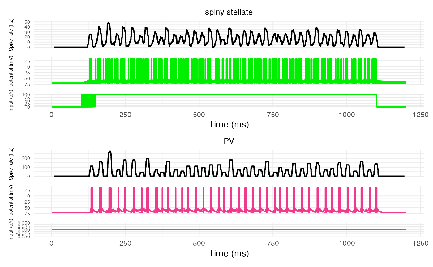
plot.network.spikerate.spectrum(network.node, max_freq = 100)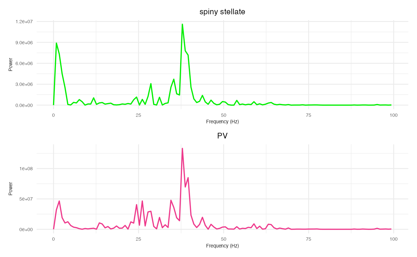
plt <- plot.network(
    network.node,
    arbor_density = 1.0,
    threedim      = TRUE
  )
plt$plot
At first glance, we see a rhythmic firing of the excitatory spiny stellates of about 4 Hz (i.e., theta waves, as in deep sleep). We see a matching rhythmic pattern for the PV cells. This is a classic excitatory-inhibitory feedback loop, wherein the excitatory cells drive the stimulus-free inhibitory cells to fire, the inhibitory firing silences the excitatory cells, which silences the inhibitory cells, allowing the stimulus current to the excitatory cells to drive them again, producing a new round of firing.
One way to see this dynamic is to rerun the simulation, first with no input into the PV cells, then with input into the PV cells, but no feedback onto the spiny stellates. Cell type information is saved across the session, so, we only need to modify the relevant part of the PV cells (the strength of the synapses from spiny stellates).
set.seed(12345)
network.node_disconnectedPV <- new.network()

# Disconnect PVs from spiny stellates
modify.cell.type(
    "PV",
    g_syn = list("spiny stellate" = 0.0)
  )

# Set network
network.node_disconnectedPV <- set.network.structure(
    network.node_disconnectedPV,
    neuron_types          = c("spiny stellate", "PV"),
    neurons_per_node      = c(n_ss, n_PV),
    synaptic_neighborhood = sn # microns
  )

# Rerun with PVs disconnected
sim_results_disconnectedPV <- run.BGT(
    network.node_disconnectedPV,
    I_stim,
    dt
  )

# Plot traces
plot.network.traces(network.node_disconnectedPV, I_stim = I_stim)
## Warning: Removed 174 rows containing missing values or values outside the scale range (`geom_line()`).
## Removed 174 rows containing missing values or values outside the scale range (`geom_line()`).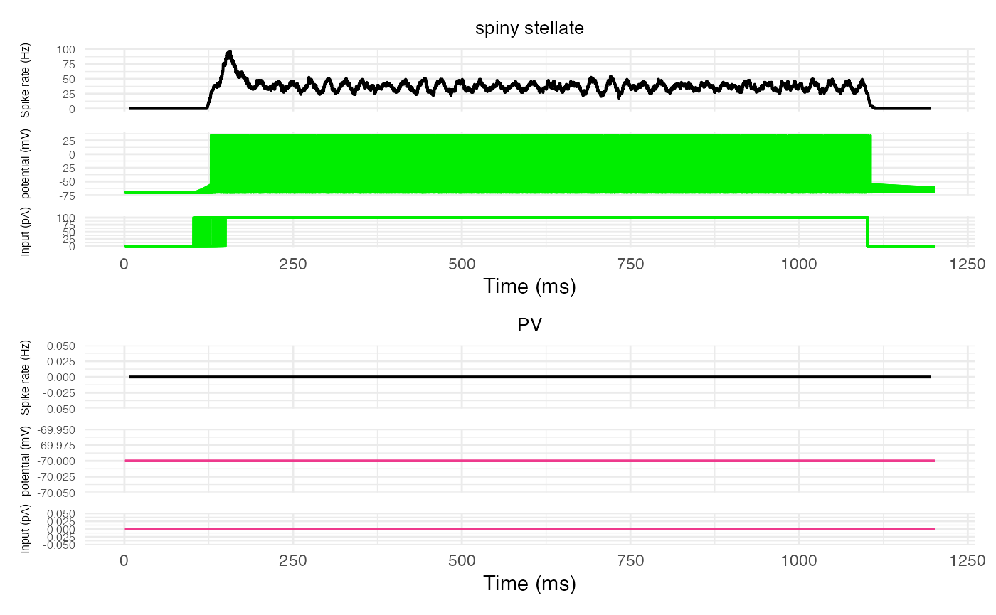
plot.network.spikerate.spectrum(network.node_disconnectedPV, max_freq = 100)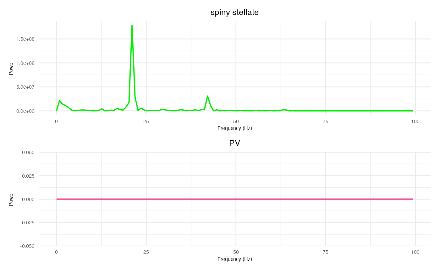
As can be seen, without spike input from the spiny stellates, the PV cells show no activity. Note, also, that without the inhibitory feedback from the PV cells, the spiny stellate population has lost its rhythmic firing. As there is a constant stimulus driving the cells, the population as a whole shows a constant firing.
Thus, the rhythmic firing pattern of the original network requires the excitatory-inhibitory feedback loop.