Single-cell temporal dynamics
Michael Barkasi
August 19, 2026 (v1.1)
tutorial_membrane_temporal_dynamics.Rmd
Introduction
Single-cell network
Let’s set up the R environment by clearing the workspace, setting a random-number generator seed, and loading the DACx package.
# Clear the R workspace to start fresh
rm(list = ls())

# Set seed for reproducibility
set.seed(12345)

# Load DACx package
library(DACx, quietly = TRUE)
Next, we create a new network object with the new.network function.
nonspiking_cell <- new.network()Set up cell
The parameters defining cell types in DACx are mostly biophysically interpretable and can be set with, or tested against, experimental data.
Parameters for transmitter type
- Valence: 1 for excitatory cells, -1 for inhibitory cells. Code variable: valence.
Temporal modulation parameters
The temporal modulation term T controlling the responsiveness (size) of \partial v/\partial t is determined by an exponential decay function with parameters:
- Temporal modulation bias: The baseline value b of T, in ms. Code variable: temporal_modulation_bias.
- Temporal modulation time constant: The time constant \tau of the exponential decay in T, in ms. Code variable: temporal_modulation_timeconstant.
- Temporal modulation amplitude: The amplitude A of the exponential decay in T, in ms. Code variable: temporal_modulation_amplitude. A value >0 induces bursting behavior, while a value of zero induces tonic (rhythmic) firing.
Development note: The values of these parameters are 1/0.0001 times the intended values in ms, due to debugging.
Intercell transmission parameters
- Transmission velocity: The speed of the action potential between neurons, in microns/ms. Code variable: transmission_velocity.
- Spine density: The proportion (a value between 0 and 1) of dendrite nodes expected to be spines. Code variable: spine_density.
- Axon target: The kind of nodes onto which the cell’s axons can synapse. Possible values include “spine”, “dendrite_shaft”, “soma”, and “axon_shaft”. Code variable axon_target.
Membrane parameters
- Potential bound: The maximum absolute value v_\mathrm{bound} of potential difference in electrical charge between the inside and outside of the cell, in mV. Code variable v_bound. Theoretically, we assume this is the absolute value of the rest voltage, plus a little bit. What matters is that -v_\mathrm{bound} \leq v \leq v_\mathrm{bound} for all possible membrane potentials v. For example, 75mV is a reasonable value.
- Metabolic energy derivative bound: Bound \partial I_\mathrm{influx} on the absolute value of the derivative \partial\mathcal{H}/\partial v of metabolic energy \mathcal{H} with respect to potential v, such that \partial I_\mathrm{influx} \geq |\partial\mathcal{H}/\partial v|, in mA. Code variable: dHdv_bound. Theoretically, we assume that this value is approximately the change in current when v crosses the spike threshold, which we assume is approximately the spike current. In practice, we add 5%.
- Spike current: The current of the action potential, i.e., the total current crossing the membrane over the entire area of the cell during a spike, in mA. Code variable: I_spike. As a starting point, we assume this is 10^{-3}mA, i.e., one mico amp.
- Spike potential: The value v_\mathrm{spike} of an action potential, in mV. Code variable: spike_potential. The default is 35mV.
- Resting potential: The potential difference v_\mathrm{rest} in electrical charge between the inside and outside of the cell at rest, in mV. Code variable: resting_potential. The default is -70mV.
- Threshold: The potential difference v_\mathrm{threshold} in electrical charge between the inside and outside of the cell at which an action potential is triggered, in mV. Code variable: threshold. The default is -55mV.
Parameters for process size and structure
- Axon branch count: An integer value giving the expected number of nodes per branch in the axon arbor. Code variable: axon_branch_count.
- Dendrite branch count: Same as axon branch count, but for dendrites. Code variable: dendrite_branch_count.
- Branch independence: The expected proportion (a value between 0 and 1) of branches which connect directly to the soma, with 1 meaning all branches connect directly to the soma and zero meaning that all branches connect to the soma from a single segment. Code variable: branch_independence.
- Branch spread: Scaled value between 0 and 1 controlling the tendency of arbor branches to repel away from the soma with 1 meaning a straight line away from the soma and 0 meaning no bias with respect to soma position. Code variable: branch_spread.
Apical dendrite parameters
- Apical target layer: Character string giving the name of the layer to which apical dendrite is expected to grow, if any; if none, “none”. Intended for modeling the circuit topology of pyramidal neurons. Code variable: apical_target_layer.
# The formula is: = v_traces.col(t - 1) + (STD_W.array() * dvdt.array() / tau.array()).matrix();
# So, the temporal modulation factor T is really STD_W/tau, where tau is a fast-response adaptation (e.g., for bursting) dependent on only time since last spike, and STD_W is a mesoscale adaptation ("short-term depression") dependent on some back-looking window of spikes.
# T(t) models ion channel kinetics (from ChatGPT): "T(t) is analogous to an effective membrane time-scale or effective membrane resistance in that it modulates the rate of voltage evolution without altering the underlying energy landscape."


modify.cell.type(
    "neuron",
    "subthreshold only",
    v_bound     = 2.0,
    g_leak      = 1.5,   # nS, Slow leak for demonstration purposes
    v_threshold = 1000   # Something large, to suppress spiking
  )

nonspiking_cell <- set.network.structure(
    nonspiking_cell,
    neuron_types     = c("subthreshold only"),
    neurons_per_node = 1
  )
BGT simulations
This gives us the number of rows needed in our stimulus current matrix. For the number of columns, we need to know the number of time steps required:
stim_time_ms <- 1000
dt           <- 1e-3
n_steps      <- stim_time_ms/dt
cat("Number of time steps in the simulation:", n_steps)
## Number of time steps in the simulation: 1e+06Now, suppose we want our simulation to involve a 20ms input current to just the spiny stellates, starting at 10ms. We can compute the initial and final time steps of this current, plus a mask for the spiny stellates, as follows:
A final question is how much current to apply. For this simulation, we’ll use a constant current of 100 pico amp (100\times 10^{-9}mA) to the spiny stellates during the stimulus period. It might be natural to leave the input current at zero outside of the stimulus period, but there is endogenous background activity even without exogenous input to the network. So, we’ll specify a baseline input current of 10 pico amps (10\times 10^{-9}mA) to all neurons throughout the entire stimulation period:
stim_magnitude <- 100
no_stim  <- matrix(0, nrow = 1, ncol = n_steps)
With the stimulus current matrix in hand, we can run the simulation:
nonspiking_cell_results <- run.BGT(
    nonspiking_cell,
    no_stim,
    dt,
    v_initial = 0.0
  )
plot.network.traces(nonspiking_cell, I_stim = no_stim, plot_rates = FALSE)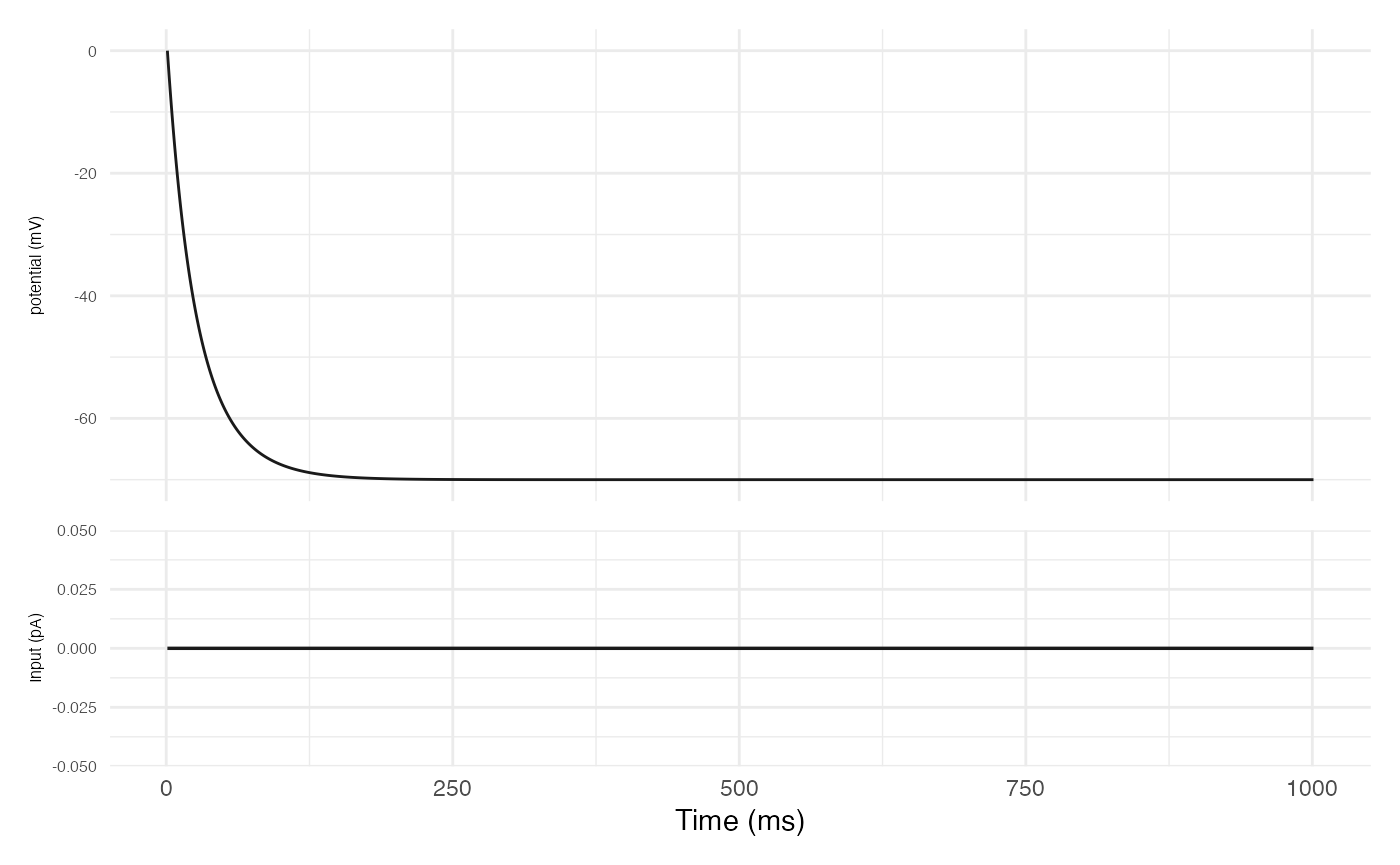
integrating_cell <- new.network()
modify.cell.type(
    "neuron",
    "leaky integrator",
    # Membrane kinetics
    tau_fast              = 1.0,   # ms
    tau_slow              = 60.0,  # ms
    tau_Vs                = 100.0, # ms/spike
    dCdr                  = 0.01,  # concentration/spike
    dVdr                  = 0.05,  # concentration/spike
    max_spike_rate        = 0.1,   # spikes/ms
    g_leak                = 1.0,   # nS
    # Intercell transmission
    spike_velocity        = 500,   # micons/ms, = 0.5 m/s
    spine_density         = 0.0,
    axon_target           = "dendrite_shaft",
    # Spiking
    I_spike               = 1e3,   # pA
    dHdv_bound            = 1.05,
    v_spike               = 35,    # mV
    tau_spike             = 1.0,   # ms
    v_threshold           = -55,   # mV
    v_eq                  = list ( # mV
      "spiny stellate" = 0.0,    # Excitatory, so drives postsynaptic cell membrane v up
      "PV"             = -80.0), # Inhibitory, so drives postsynaptic cell membrane v down
    # Membrane characteristics
    v_rest                = -70,   # mV
    v_bound               = 1.15,
    g_syn                 = list(  # nS
      "spiny stellate" = 0.1,
      "PV"             = 0.1),
    tau_syn               = list(  # ms
      "spiny stellate" = 2.0,   # Excitatory glutamate channels close quickly
      "PV"             = 6.0),  # Inhibitory GABA channels stay open longer
    # Neurite structure
    axon_branch_count     = 20,
    dendrite_branch_count = 20,
    branch_independence   = 0.75,
    branch_spread         = 0.75,
    apical_target_layer   = "none"
  )


integrating_cell <- set.network.structure(
    integrating_cell,
    neuron_types     = c("leaky integrator"),
    neurons_per_node = 1
  )
# Set stimulus start and length
stim_length_ms <- 5
stim_start_ms  <- seq(from = 50, to = 950, by = 100)
# Find start and end steps of the input stimulus current
stim_length    <- stim_length_ms / dt
stim_start     <- stim_start_ms / dt
stim_end       <- stim_start + stim_length - 1
short_stims    <- no_stim
for (i in seq_along(stim_start)) {
  short_stims[, stim_start[i]:stim_end[i]] <- stim_magnitude
}
integrating_cell_results <- run.BGT(
  integrating_cell,
  short_stims,
  dt,
  v_initial = -70
)
plot.network.traces(integrating_cell, I_stim = short_stims, plot_rates = FALSE)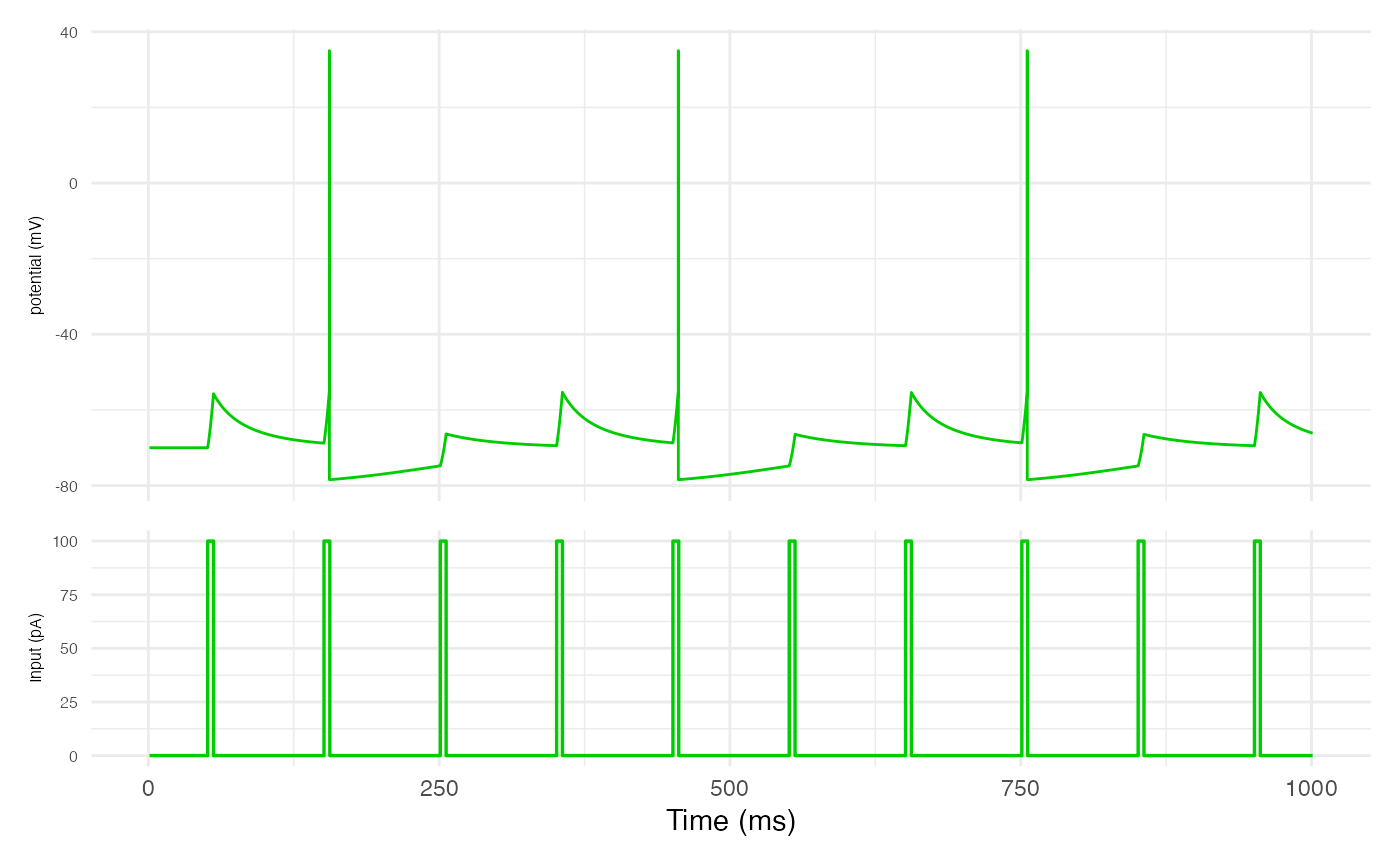
bursting_cell <- new.network()
modify.cell.type(
    "leaky integrator",
    "bursting cell",
    dCdr = 0.09, # up from 0.01, to induce bursting
  )

bursting_cell <- set.network.structure(
    bursting_cell,
    neuron_types = c("bursting cell"),
    neurons_per_node = 1
  )
# Set stimulus start and length
stim_length_ms <- 100
stim_start_ms  <- seq(from = 100, to = 750, by = 200)
# Find start and end steps of the input stimulus current
stim_length    <- stim_length_ms / dt
stim_start     <- stim_start_ms / dt
stim_end       <- stim_start + stim_length - 1
long_stims     <- no_stim
for (i in seq_along(stim_start)) {
  long_stims[, stim_start[i]:stim_end[i]] <- stim_magnitude
}
bursting_cell_results <- run.BGT(
  bursting_cell,
  long_stims,
  dt,
  v_initial = -70
)
plot.network.traces(bursting_cell, I_stim = long_stims, plot_rates = FALSE)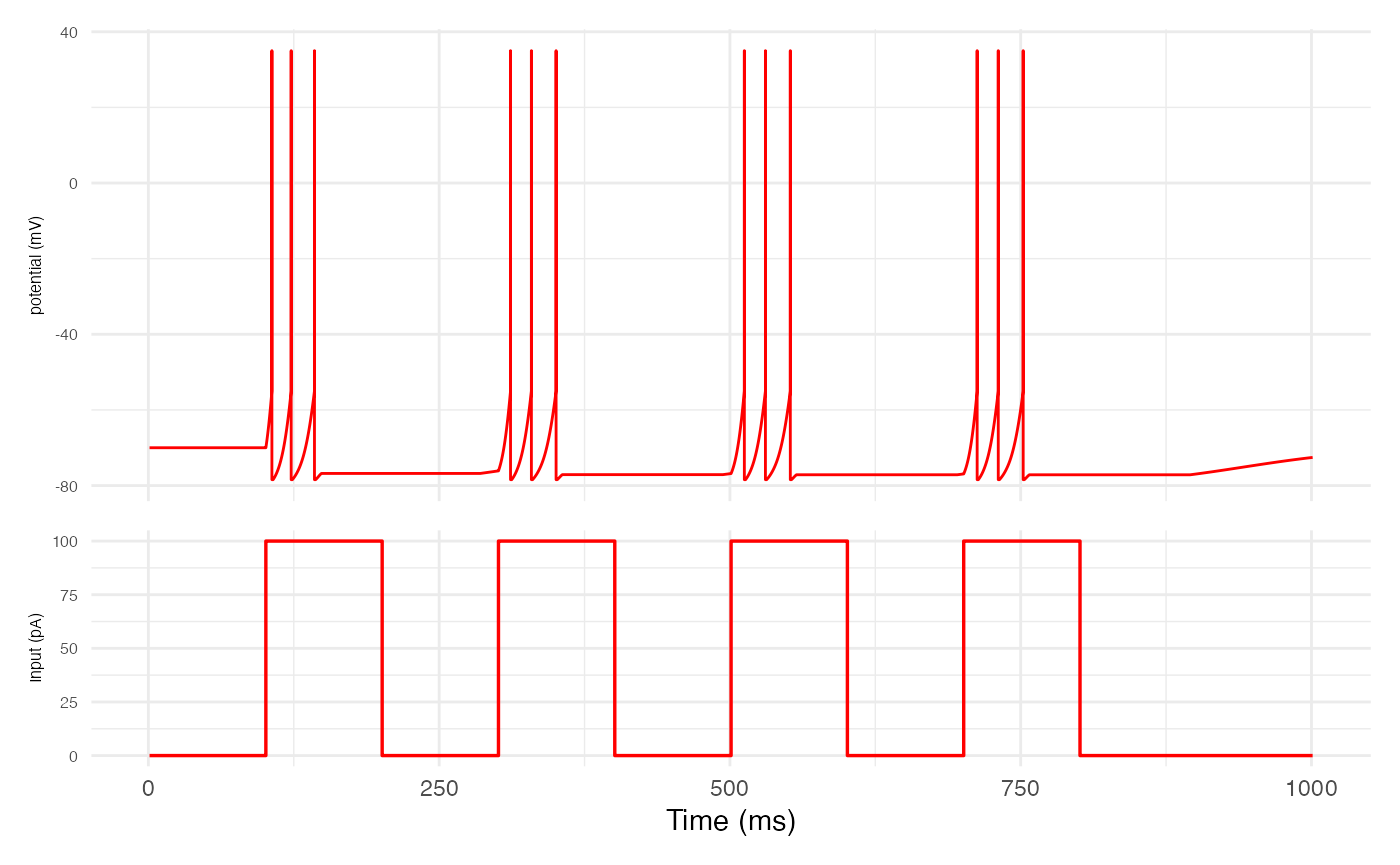
integrating_cell_results <- run.BGT(
  integrating_cell,
  long_stims,
  dt,
  v_initial = -70
)
plot.network.traces(integrating_cell, I_stim = long_stims, plot_rates = FALSE)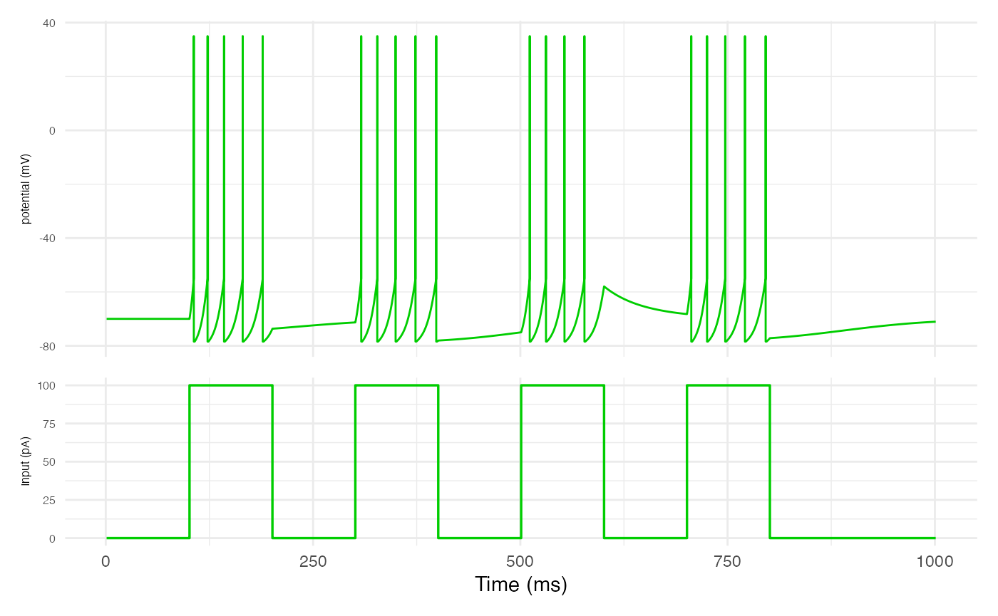
# Set stimulus start and length
stim_length_ms  <- 800
stim_start_ms   <- 100
# Find start and end steps of the input stimulus current
stim_length     <- stim_length_ms / dt
stim_start      <- stim_start_ms / dt
stim_end        <- stim_start + stim_length - 1
continuous_stim <- no_stim
for (i in seq_along(stim_start)) {
  continuous_stim[, stim_start[i]:stim_end[i]] <- stim_magnitude
}
network_both <- new.network()
network_both <- set.network.structure(
    network_both,
    neuron_types = c("bursting cell", "leaky integrator"),
    neurons_per_node = 1
  )
no_stim2  <- matrix(0, nrow = 2, ncol = n_steps)
continuous_stim2 <- no_stim2
for (i in seq_along(stim_start)) {
  continuous_stim2[, stim_start[i]:stim_end[i]] <- stim_magnitude
}
network_both_long <- run.BGT(
  network_both,
  continuous_stim2,
  dt,
  v_initial = -70
)
plot.network.traces(
  network_both,
  I_stim = continuous_stim2,
  plot_rates   = TRUE,
  window_size  = 0.1,
  return_plot  = TRUE
  )
## Warning: Removed 49998 rows containing missing values or values outside the scale range (`geom_line()`).
## Removed 49998 rows containing missing values or values outside the scale range (`geom_line()`).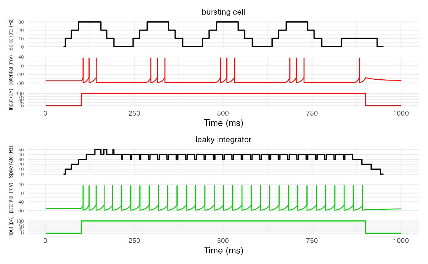
modify.cell.type(
    "leaky integrator",
    "slow recovery",
    tau_Vs = 500.0 # up from 100.0
  )
modify.cell.type(
    "leaky integrator",
    "slow drain",
    dVdr = 0.01 # down from 0.05
  )
network_both <- new.network()
network_both <- set.network.structure(
    network_both,
    neuron_types = c("leaky integrator", "slow recovery", "slow drain"),
    neurons_per_node = 1
  )

# Set stimulus start and length
stim_length_ms  <- 1200
stim_start_ms   <- 100
# Find start and end steps of the input stimulus current
stim_length     <- stim_length_ms / dt
stim_start      <- stim_start_ms / dt
stim_end        <- stim_start + stim_length - 1
no_stim2          <- matrix(0, nrow = 3, ncol = stim_end + (100/dt))
continuous_stim2  <- no_stim2
recover_start_ms  <- c(200, 500)
recover_length_ms <- c(100, 500)
recover_start     <- recover_start_ms / dt
recover_length    <- recover_length_ms / dt
recover_end       <- recover_start + recover_length - 1
for (i in seq_along(stim_start)) {
  continuous_stim2[, stim_start[i]:stim_end[i]] <- stim_magnitude
}
for (i in seq_along(recover_start)) {
  continuous_stim2[, recover_start[i]:recover_end[i]] <- 0
}
network_both_long <- run.BGT(
  network_both,
  continuous_stim2,
  dt,
  v_initial = -70
)
plt <- plot.network.traces(network_both, I_stim = continuous_stim2, plot_rates = TRUE, window_size = 0.05, return_plot = TRUE)
plt <- plt & ggplot2::theme(
            plot.title       = ggplot2::element_text(hjust = 0.5, size = 14),
            axis.title.y     = ggplot2::element_text(size = 10),
            axis.text.y      = ggplot2::element_text(size = 8)
          )
for (p in c(1:3)) {
  plt[[p]][[1]] <- plt[[p]][[1]] + ggplot2::coord_cartesian(ylim = c(0, 120)) +
  ggplot2::geom_hline(
    yintercept = 75,
    color = "red",
    linetype = "dashed"
  )
}
Temporal modulation
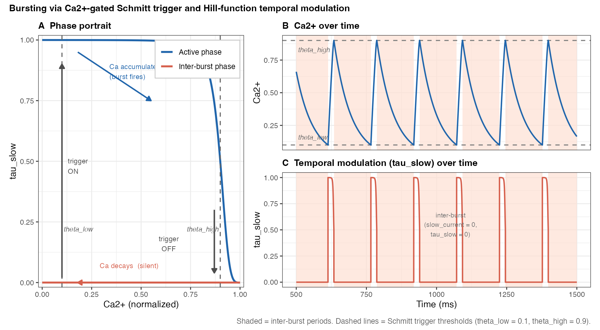
The final step in GT models (including BGT models) is to divide the rate of change for membrane potential \partial v/\partial t by a temporal modulation term T, such that: v(t+1) = v(t) + \frac{\left.\frac{\partial v}{\partial t}\right|_{t+1}}{T} This term T is given by the following exponential decay model: T = b + A\exp\left(-\frac{x}{\tau}\right) where b is the temporal modulation bias, A is the temporal modulation amplitude, and \tau is the temporal modulation time constant. The traditional input x is filled by B, a “burst” step counter. The step counter B is merely a numerical device in the simulation to carry T repeatedly across the exponential decay via the input x. When T<b, B resets to zero (and thus T jumps again to a high number), resetting the exponential decay.
When the amplitude A is zero, the exponential decay has no effect and all that’s relevant is the bias b. When A>0, the effect is to increase T at the start of the step counter, thereby shrinking the effect of \partial v/\partial t. This shrinkage follows the exponential decay of T, so that there is little chance in v (i.e., small \partial v/\partial t) at the start of the step counter, but the possibility for large changes in v at the end of the step counter. Thus, when at the end of the step counter, neurons are prone to many spikes as their membrane potential rapidly changes, creating a bursting effect.
##
## Attaching package: 'dplyr'
## The following objects are masked from 'package:stats':
##
## filter, lag## The following objects are masked from 'package:base':
##
## intersect, setdiff, setequal, union
library(ggplot2)

# Parameters matching DACx.cpp BGT simulation
theta_low  <- 0.1
theta_high <- 0.9
theta_n    <- theta_low^4   # places Hill midpoint at Ca = theta_high
tau_slow   <- 60            # ms, Ca2+ decay time constant
dCdr_eff   <- 0.05          # Ca2+ influx per unit tau_slow_effect
dt_plot    <- 0.1           # ms, step size for this illustrative simulation

# Analytical curves: tau_slow_effect vs Ca2+ for each Schmitt trigger state
Ca_seq   <- seq(0, 1, by = 0.001)
df_phase <- bind_rows(
  tibble(Ca  = Ca_seq,
         tau = (1 - Ca_seq)^4 / ((1 - Ca_seq)^4 + theta_n),
         phase = "Active (slow_current = 1)"),
  tibble(Ca  = Ca_seq,
         tau = 0,
         phase = "Inter-burst (slow_current = 0)")
)

# Simplified Ca2+ dynamics simulation
n_sim <- 60000L
Ca_sim  <- numeric(n_sim)
tau_sim <- numeric(n_sim)
sc_sim  <- logical(n_sim)
Ca_sim[1] <- 0
sc_sim[1] <- TRUE
for (t in 2:n_sim) {
  sc       <- sc_sim[t - 1]
  Ca       <- Ca_sim[t - 1]
  Ca_n     <- (as.numeric(sc) - Ca)^4
  tau_se   <- as.numeric(sc) * Ca_n / (Ca_n + theta_n)
  tau_sim[t - 1] <- tau_se
  Ca_new   <- Ca + (dCdr_eff * tau_se - Ca / tau_slow) * dt_plot
  Ca_sim[t] <- max(0, Ca_new)
  if      ( sc && Ca_new >= theta_high) sc_sim[t] <- FALSE
  else if (!sc && Ca_new <= theta_low)  sc_sim[t] <- TRUE
  else                                  sc_sim[t] <- sc
}
Ca_n_last    <- (as.numeric(sc_sim[n_sim]) - Ca_sim[n_sim])^4
tau_sim[n_sim] <- as.numeric(sc_sim[n_sim]) * Ca_n_last / (Ca_n_last + theta_n)
t_ms_sim <- (seq_len(n_sim) - 1) * dt_plot

# Select a representative window with ~6 burst cycles (after transient settles)
win_start <- 500
win_end   <- 1500
idx    <- which(t_ms_sim >= win_start & t_ms_sim <= win_end)
df_ts  <- tibble(t = t_ms_sim[idx], Ca = Ca_sim[idx],
                 tau = tau_sim[idx], sc = sc_sim[idx])

# Identify inter-burst intervals for shading
runs      <- rle(df_ts$sc)
grp_end   <- cumsum(runs$lengths)
grp_start <- c(1, grp_end[-length(grp_end)] + 1)
shade_df  <- tibble(sc    = runs$values,
                    t_min = df_ts$t[grp_start],
                    t_max = df_ts$t[grp_end]) |>
  filter(!sc)

# Panel A: Phase portrait (analytical)
p_phase3 <- ggplot() +
  geom_line(data = df_phase, aes(x = Ca, y = tau, color = phase), linewidth = 1.1) +
  geom_vline(xintercept = theta_low,  linetype = "dashed", color = "gray40", linewidth = 0.6) +
  geom_vline(xintercept = theta_high, linetype = "dashed", color = "gray40", linewidth = 0.6) +
  annotate("segment", x=0.18, xend=0.55, y=0.95, yend=0.75,
           arrow=arrow(length=unit(0.2,"cm"), type="closed"), color="#2166ac", linewidth=0.8) +
  annotate("segment", x=0.87, xend=0.87, y=0.30, yend=0.04,
           arrow=arrow(length=unit(0.2,"cm"), type="closed"), color="gray30",  linewidth=0.8) +
  annotate("segment", x=0.73, xend=0.18, y=0,    yend=0,
           arrow=arrow(length=unit(0.2,"cm"), type="closed"), color="#d6604d", linewidth=0.8) +
  annotate("segment", x=0.1,  xend=0.1,  y=0.02, yend=0.90,
           arrow=arrow(length=unit(0.2,"cm"), type="closed"), color="gray30",  linewidth=0.8) +
  annotate("text", x=0.34, y=0.87, label="Ca accumulates\n(burst fires)", size=3.0, color="#2166ac", hjust=0) +
  annotate("text", x=0.64, y=0.16, label="trigger\nOFF",                  size=3.0, color="gray30",  hjust=0.5) +
  annotate("text", x=0.44, y=0.07, label="Ca decays  (silent)",           size=3.0, color="#d6604d", hjust=0.5) +
  annotate("text", x=0.13, y=0.48, label="trigger\nON",                   size=3.0, color="gray30",  hjust=0) +
  annotate("text", x=theta_low,  y=0.22, label="theta_low",  size=2.9, color="gray35", hjust=-0.05, fontface="italic") +
  annotate("text", x=theta_high, y=0.22, label="theta_high", size=2.9, color="gray35", hjust= 1.05, fontface="italic") +
  scale_color_manual(
    values = c("Active (slow_current = 1)"     = "#2166ac",
               "Inter-burst (slow_current = 0)" = "#d6604d"),
    labels = c("Active phase", "Inter-burst phase")
  ) +
  scale_x_continuous(limits = c(0, 1), expand = c(0.02, 0)) +
  scale_y_continuous(limits = c(0, 1.0), expand = c(0.01, 0.01)) +
  labs(title = "A  Phase portrait",
       x = "Ca2+ (normalized)", y = "tau_slow", color = NULL) +
  theme_bw(base_size = 11) +
  theme(legend.position     = c(0.98, 0.98),
        legend.justification = c(1, 1),
        legend.background   = element_rect(fill = "white", color = "gray80"),
        legend.text         = element_text(size = 9),
        plot.title          = element_text(face = "bold", size = 11))

# Panel B: Ca2+ over time
p_ca3 <- ggplot(df_ts, aes(x = t, y = Ca)) +
  geom_rect(data = shade_df,
            aes(xmin = t_min, xmax = t_max, ymin = -Inf, ymax = Inf),
            inherit.aes = FALSE, fill = "#fee0d2", alpha = 0.7) +
  geom_hline(yintercept = theta_low,  linetype = "dashed", color = "gray50", linewidth = 0.6) +
  geom_hline(yintercept = theta_high, linetype = "dashed", color = "gray50", linewidth = 0.6) +
  geom_line(color = "#2166ac", linewidth = 0.8) +
  annotate("text", x=win_start+5, y=theta_low +0.06, label="theta_low",  size=2.9, color="gray40", hjust=0, fontface="italic") +
  annotate("text", x=win_start+5, y=theta_high-0.07, label="theta_high", size=2.9, color="gray40", hjust=0, fontface="italic") +
  labs(title = "B  Ca2+ over time", x = NULL, y = "Ca2+") +
  theme_bw(base_size = 11) +
  theme(plot.title   = element_text(face = "bold", size = 11),
        axis.text.x  = element_blank(),
        axis.ticks.x = element_blank())

# Panel C: tau_slow over time
p_tau3 <- ggplot(df_ts, aes(x = t, y = tau)) +
  geom_rect(data = shade_df,
            aes(xmin = t_min, xmax = t_max, ymin = -Inf, ymax = Inf),
            inherit.aes = FALSE, fill = "#fee0d2", alpha = 0.7) +
  geom_line(color = "#d6604d", linewidth = 0.8) +
  annotate("text", x=1050, y=0.55,
           label="inter-burst\n(slow_current = 0,\ntau_slow = 0)",
           size=2.8, color="gray45", hjust=0.5) +
  labs(title = "C  Temporal modulation (tau_slow) over time",
       x = "Time (ms)", y = "tau_slow") +
  theme_bw(base_size = 11) +
  theme(plot.title = element_text(face = "bold", size = 11))

# Combine panels
p_phase3 + (p_ca3 / p_tau3) +
  plot_layout(widths = c(1, 1.5)) +
  plot_annotation(
    title   = "Bursting via Ca2+-gated Schmitt trigger and Hill-function temporal modulation",
    caption = paste("Shaded = inter-burst periods. Dashed lines = Schmitt trigger thresholds",
                    "(theta_low = 0.1, theta_high = 0.9)."),
    theme   = theme(plot.title   = element_text(size = 11, face = "bold"),
                    plot.caption = element_text(size = 9,  color = "gray40"))
  )
p_phase3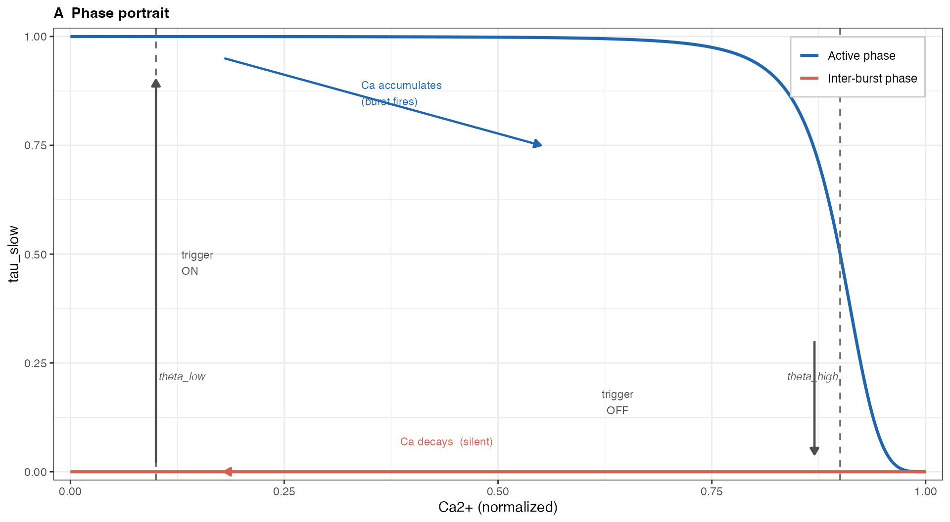
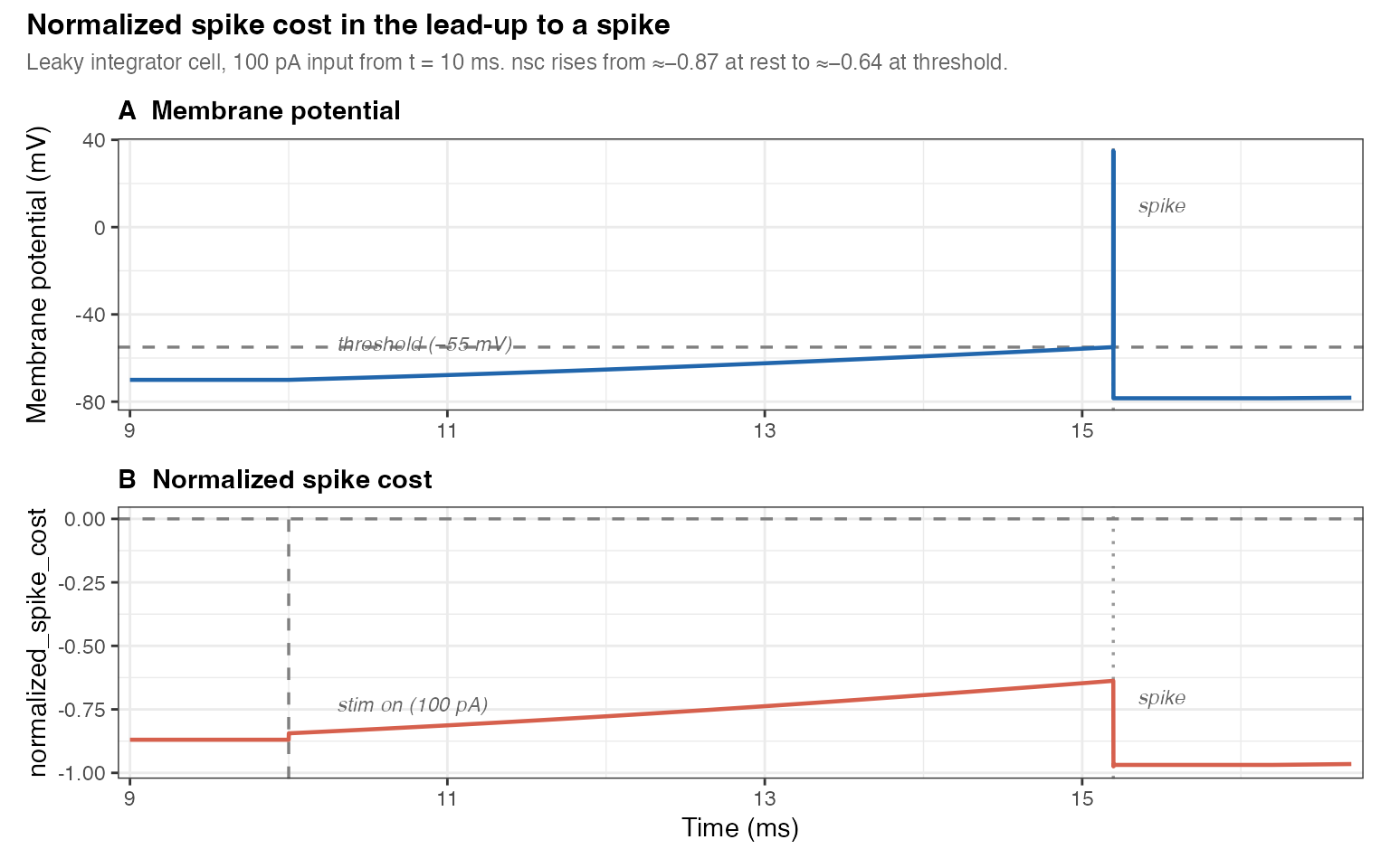
Normalized spike cost in the lead-up to a spike
The quantity normalized_spike_cost (DACx.cpp, line 2514)
is the energetic heart of the BGT spike-generation mechanism. It is
defined as
\text{nsc}(t) = \frac{\overbrace{\partial\mathcal{H}_{\max} \cdot v(t)}^{\text{spike initiation power}} - \overbrace{\left.\frac{\partial\mathcal{H}}{\partial v}\right|_t \cdot v_{\text{bound}}}^{\text{rest maintenance power}}}{\underbrace{\partial\mathcal{H}_{\max} \cdot v_{\text{bound}}}_{\text{max initiation power from rest}} - \underbrace{\left.\frac{\partial\mathcal{H}}{\partial v}\right|_t \cdot v(t)}_{\text{maintenance power at current } v}}
where \partial\mathcal{H}/\partial v captures the net current balance at the membrane (synaptic + leak + stimulus + any ongoing spike current) and \partial\mathcal{H}_{\max} is its bound. The quantity nsc \in [-1, 1], where \text{nsc} = -1 corresponds to maximum hyperpolarization and \text{nsc} = 1 to maximum depolarization or maximum inward current.
nsc as an attractor. The raw rate of change of membrane potential is set as \partial v/\partial t = v_{\text{bound}} \cdot \text{nsc} - v, making v_{\text{bound}} \cdot \text{nsc} an attractor voltage toward which the membrane is continuously pulled. The temporal modulation term T (line 2526) then scales this raw \partial v/\partial t by T \cdot \Delta t, controlling the rate of movement toward the attractor independently of the attractor’s position. This cleanly separates the energetic direction of membrane dynamics (determined by nsc) from the kinetic rate of those dynamics (determined by T via spike history and calcium).
Energetic interpretation. The sign of nsc reflects a metabolic cost comparison: \text{nsc} < 0 means spike initiation is energetically cheaper than maintaining the current subthreshold state — the cell is continuously being pulled toward a spike. Under physiological depolarizing input this holds throughout the charging phase, with nsc rising (becoming less negative) as the membrane approaches threshold. The voltage threshold itself plays a secondary role: it only determines when the spike current I_\text{spike} enters the \partial\mathcal{H}/\partial v calculation, sharply increasing the outward current and collapsing nsc post-spike. Spiking in this model is therefore not a threshold-crossing rule but the outcome of continuous energetic accounting: the membrane moves toward the spike because that is the lower-energy trajectory.
The block below runs a leaky integrator cell (same parameters as the
tutorial) with a constant 100 pA input, reconstructs
normalized_spike_cost from the voltage trace, and plots it
alongside the membrane potential in the lead-up to the first spike.
library(DACx)
library(ggplot2)
library(patchwork)

# ── 1. Build a leaky integrator network (tutorial parameters) ──────────────────
nsc_cell <- new.network()
modify.cell.type(
  "neuron", "leaky integrator",
  tau_fast              = 1.0,    # ms
  tau_slow              = 60.0,   # ms
  tau_Vs                = 100.0,  # ms/spike
  dCdr                  = 0.01,   # concentration/spike
  dVdr                  = 0.05,   # concentration/spike
  max_spike_rate        = 0.1,    # spikes/ms
  g_leak                = 1.0,    # nS
  spike_velocity        = 500,    # microns/ms
  spine_density         = 0.0,
  axon_target           = "dendrite_shaft",
  I_spike               = 1e3,    # pA
  dHdv_bound            = 1.05,
  v_spike               = 35,     # mV
  tau_spike             = 1.0,    # ms
  v_threshold           = -55,    # mV
  v_eq                  = list("spiny stellate" = 0.0, "PV" = -80.0),
  v_rest                = -70,    # mV
  v_bound               = 1.15,
  g_syn                 = list("spiny stellate" = 0.1, "PV" = 0.1),
  tau_syn               = list("spiny stellate" = 2.0, "PV" = 6.0),
  axon_branch_count     = 20,
  dendrite_branch_count = 20,
  branch_independence   = 0.75,
  branch_spread         = 0.75,
  apical_target_layer   = "none"
)
nsc_cell <- set.network.structure(
  nsc_cell,
  neuron_types     = c("leaky integrator"),
  neurons_per_node = 1
)

# ── 2. Stimulus: 100 pA constant input starting at 10 ms ──────────────────────
dt_nsc    <- 1e-3          # ms
sim_ms    <- 25            # ms (captures first spike)
n_steps   <- sim_ms / dt_nsc
I_nsc     <- matrix(0, nrow = 1, ncol = n_steps)
I_nsc[, round(10 / dt_nsc):n_steps] <- 100  # pA

# ── 3. Run BGT simulation ──────────────────────────────────────────────────────
run.BGT(nsc_cell, I_nsc, dt_nsc, v_initial = -70)
## $v_traces
## [,1] [,2] [,3] [,4] [,5] [,6] [,7] [,8] [,9] [,10] [,11] [,12] [,13] [,14] [,15] [,16] [,17] [,18] [,19] [,20] [,21] [,22] [,23] [,24] [,25] [,26] [,27] [,28] [,29] [,30] [,31] [,32] [,33] [,34] [,35] [,36] [,37] [,38] [,39] [,40] [,41] [,42] [,43] [,44] [,45] [,46] [,47] [,48] [,49] [,50] [,51] [,52] [,53] [,54] [,55] [,56] [,57] [,58] [,59] [,60] [,61] [,62] [,63] [,64] [,65] [,66] [,67] [,68] [,69] [,70] [,71] [,72] [,73] [,74] [,75] [,76] [,77] [,78] [,79] [,80] [,81] [,82] [,83] [,84] [,85] [,86] [,87] [,88] [,89] [,90] [,91] [,92] [,93] [,94] [,95] [,96] [,97] [,98] [,99] [,100] [,101] [,102] [,103] [,104] [,105] [,106] [,107] [,108] [,109] [,110] [,111] [,112] [,113] [,114] [,115] [,116] [,117] [,118] [,119] [,120] [,121] [,122] [,123] [,124] [,125] [,126] [,127] [,128] [,129] [,130] [,131] [,132] [,133] [,134] [,135] [,136] [,137] [,138] [,139] [,140] [,141] [,142] [,143] [,144] [,145] [,146] [,147] [,148] [,149] [,150] [,151] [,152] [,153] [,154] [,155] [,156] [,157] [,158] [,159] [,160] [,161] [,162] [,163] [,164] [,165] [,166] [,167] [,168] [,169] [,170] [,171] [,172] [,173] [,174] [,175] [,176] [,177] [,178] [,179] [,180] [,181] [,182] [,183] [,184] [,185] [,186] [,187] [,188] [,189] [,190] [,191] [,192] [,193] [,194] [,195] [,196] [,197] [,198] [,199] [,200] [,201] [,202] [,203] [,204] [,205] [,206] [,207] [,208] [,209] [,210] [,211] [,212] [,213] [,214] [,215] [,216] [,217] [,218] [,219] [,220] [,221] [,222] [,223] [,224] [,225] [,226] [,227] [,228] [,229] [,230] [,231] [,232] [,233] [,234] [,235] [,236] [,237] [,238] [,239] [,240] [,241] [,242] [,243] [,244] [,245] [,246] [,247] [,248] [,249] [,250] [,251] [,252] [,253] [,254] [,255] [,256] [,257] [,258] [,259] [,260] [,261] [,262] [,263] [,264] [,265] [,266] [,267] [,268] [,269] [,270] [,271] [,272] [,273] [,274] [,275] [,276] [,277] [,278] [,279] [,280] [,281] [,282] [,283] [,284] [,285] [,286] [,287] [,288] [,289] [,290] [,291] [,292] [,293] [,294] [,295] [,296] [,297] [,298] [,299] [,300] [,301] [,302] [,303] [,304] [,305] [,306] [,307] [,308] [,309] [,310] [,311] [,312] [,313] [,314] [,315] [,316] [,317] [,318] [,319] [,320] [,321] [,322] [,323] [,324] [,325] [,326] [,327] [,328] [,329] [,330] [,331] [,332] [,333] [,334] [,335] [,336] [,337] [,338] [,339] [,340] [,341] [,342] [,343] [,344] [,345] [,346] [,347] [,348] [,349] [,350] [,351] [,352] [,353] [,354] [,355] [,356] [,357] [,358] [,359] [,360] [,361] [,362] [,363] [,364] [,365] [,366] [,367] [,368] [,369] [,370] [,371] [,372] [,373] [,374] [,375] [,376] [,377] [,378] [,379] [,380] [,381] [,382] [,383] [,384] [,385] [,386] [,387] [,388] [,389] [,390] [,391] [,392] [,393] [,394] [,395] [,396] [,397] [,398] [,399] [,400] [,401] [,402] [,403] [,404] [,405] [,406] [,407] [,408] [,409] [,410] [,411] [,412] [,413] [,414] [,415] [,416] [,417] [,418] [,419] [,420] [,421] [,422] [,423] [,424] [,425] [,426] [,427] [,428] [,429] [,430] [,431] [,432] [,433] [,434] [,435] [,436] [,437] [,438] [,439] [,440] [,441] [,442] [,443] [,444] [,445] [,446] [,447] [,448] [,449] [,450] [,451] [,452] [,453] [,454] [,455] [,456] [,457] [,458] [,459] [,460] [,461] [,462] [,463] [,464] [,465] [,466] [,467] [,468] [,469] [,470] [,471] [,472] [,473] [,474] [,475] [,476] [,477] [,478] [,479] [,480] [,481] [,482] [,483] [,484] [,485] [,486] [,487] [,488] [,489] [,490] [,491] [,492] [,493] [,494] [,495] [,496] [,497] [,498] [,499] [,500] [,501] [,502] [,503] [,504] [,505] [,506] [,507] [,508] [,509] [,510] [,511] [,512] [,513] [,514] [,515] [,516] [,517] [,518] [,519] [,520] [,521] [,522] [,523] [,524] [,525] [,526] [,527] [,528] [,529] [,530] [,531] [,532] [,533] [,534] [,535] [,536] [,537] [,538] [,539] [,540] [,541] [,542] [,543] [,544] [,545] [,546] [,547] [,548] [,549] [,550] [,551] [,552] [,553] [,554] [,555] [,556] [,557] [,558] [,559] [,560] [,561] [,562] [,563] [,564] [,565] [,566] [,567] [,568] [,569] [,570] [,571] [,572] [,573] [,574] [,575] [,576] [,577] [,578] [,579] [,580] [,581] [,582] [,583] [,584] [,585] [,586] [,587] [,588] [,589] [,590] [,591] [,592] [,593] [,594] [,595] [,596] [,597] [,598] [,599] [,600] [,601] [,602] [,603] [,604] [,605] [,606] [,607] [,608] [,609] [,610] [,611] [,612] [,613] [,614] [,615] [,616] [,617] [,618] [,619] [,620] [,621] [,622] [,623] [,624] [,625] [,626] [,627] [,628] [,629] [,630] [,631] [,632] [,633] [,634] [,635] [,636] [,637] [,638] [,639] [,640] [,641] [,642] [,643] [,644] [,645] [,646] [,647] [,648] [,649] [,650] [,651] [,652] [,653] [,654] [,655] [,656] [,657] [,658] [,659] [,660] [,661] [,662] [,663] [,664] [,665] [,666] [,667] [,668] [,669] [,670] [,671] [,672] [,673] [,674] [,675] [,676] [,677] [,678] [,679] [,680] [,681] [,682] [,683] [,684] [,685] [,686] [,687] [,688] [,689] [,690] [,691] [,692] [,693] [,694] [,695] [,696] [,697] [,698] [,699] [,700] [,701] [,702] [,703] [,704] [,705] [,706] [,707] [,708] [,709] [,710] [,711] [,712] [,713] [,714] [,715] [,716] [,717] [,718] [,719] [,720] [,721] [,722] [,723] [,724] [,725] [,726] [,727] [,728] [,729] [,730] [,731] [,732] [,733] [,734] [,735] [,736] [,737] [,738] [,739] [,740] [,741] [,742] [,743] [,744] [,745] [,746] [,747] [,748] [,749] [,750] [,751] [,752] [,753] [,754] [,755] [,756] [,757] [,758] [,759] [,760] [,761] [,762] [,763] [,764] [,765] [,766] [,767] [,768] [,769] [,770] [,771] [,772] [,773] [,774] [,775] [,776] [,777] [,778] [,779] [,780] [,781] [,782] [,783] [,784] [,785] [,786] [,787] [,788] [,789] [,790] [,791] [,792] [,793] [,794] [,795] [,796] [,797] [,798] [,799] [,800] [,801] [,802] [,803] [,804] [,805] [,806] [,807] [,808] [,809] [,810] [,811] [,812] [,813] [,814] [,815] [,816] [,817] [,818] [,819] [,820] [,821] [,822] [,823] [,824] [,825] [,826] [,827] [,828] [,829] [,830] [,831] [,832] [,833] [,834] [,835] [,836] [,837] [,838] [,839] [,840] [,841] [,842] [,843] [,844] [,845] [,846] [,847] [,848] [,849] [,850] [,851] [,852] [,853] [,854] [,855] [,856] [,857] [,858] [,859] [,860] [,861] [,862] [,863] [,864] [,865] [,866] [,867] [,868] [,869] [,870] [,871] [,872] [,873] [,874] [,875] [,876] [,877] [,878] [,879] [,880] [,881] [,882] [,883] [,884] [,885] [,886] [,887] [,888] [,889] [,890] [,891] [,892] [,893] [,894] [,895] [,896] [,897] [,898] [,899] [,900] [,901] [,902] [,903] [,904] [,905] [,906] [,907] [,908] [,909] [,910] [,911] [,912] [,913] [,914] [,915] [,916] [,917] [,918] [,919] [,920] [,921] [,922] [,923] [,924] [,925] [,926] [,927] [,928] [,929] [,930] [,931] [,932] [,933] [,934] [,935] [,936] [,937] [,938] [,939] [,940] [,941] [,942] [,943] [,944] [,945] [,946] [,947] [,948] [,949] [,950] [,951] [,952] [,953] [,954] [,955] [,956] [,957] [,958] [,959] [,960] [,961] [,962] [,963] [,964] [,965] [,966] [,967] [,968] [,969] [,970] [,971] [,972] [,973] [,974] [,975] [,976] [,977] [,978] [,979] [,980] [,981] [,982] [,983] [,984] [,985] [,986] [,987] [,988] [,989] [,990] [,991] [,992] [,993] [,994] [,995] [,996] [,997] [,998] [,999] [,1000] [,1001] [,1002] [,1003] [,1004] [,1005] [,1006] [,1007] [,1008] [,1009] [,1010] [,1011] [,1012] [,1013] [,1014] [,1015] [,1016] [,1017] [,1018] [,1019] [,1020] [,1021] [,1022] [,1023] [,1024] [,1025] [,1026] [,1027] [,1028] [,1029] [,1030] [,1031] [,1032] [,1033] [,1034] [,1035] [,1036] [,1037] [,1038] [,1039] [,1040] [,1041] [,1042] [,1043] [,1044] [,1045] [,1046] [,1047] [,1048] [,1049] [,1050] [,1051] [,1052] [,1053] [,1054] [,1055] [,1056] [,1057] [,1058] [,1059] [,1060] [,1061] [,1062] [,1063] [,1064] [,1065] [,1066] [,1067] [,1068] [,1069] [,1070] [,1071] [,1072] [,1073] [,1074] [,1075] [,1076] [,1077] [,1078] [,1079] [,1080] [,1081] [,1082] [,1083] [,1084] [,1085] [,1086] [,1087] [,1088] [,1089] [,1090] [,1091] [,1092] [,1093] [,1094] [,1095] [,1096] [,1097] [,1098] [,1099] [,1100] [,1101] [,1102] [,1103] [,1104] [,1105] [,1106] [,1107] [,1108] [,1109] [,1110] [,1111] [,1112] [,1113] [,1114] [,1115] [,1116] [,1117] [,1118] [,1119] [,1120] [,1121] [,1122] [,1123] [,1124] [,1125] [,1126] [,1127] [,1128] [,1129] [,1130] [,1131] [,1132] [,1133] [,1134] [,1135] [,1136] [,1137] [,1138] [,1139] [,1140] [,1141] [,1142] [,1143] [,1144] [,1145] [,1146] [,1147] [,1148] [,1149] [,1150] [,1151] [,1152] [,1153] [,1154] [,1155] [,1156] [,1157] [,1158] [,1159] [,1160] [,1161] [,1162] [,1163] [,1164] [,1165] [,1166] [,1167] [,1168] [,1169] [,1170] [,1171] [,1172] [,1173] [,1174] [,1175] [,1176] [,1177] [,1178] [,1179] [,1180] [,1181] [,1182] [,1183] [,1184] [,1185] [,1186] [,1187] [,1188] [,1189] [,1190] [,1191] [,1192] [,1193] [,1194] [,1195] [,1196] [,1197] [,1198] [,1199] [,1200] [,1201] [,1202] [,1203] [,1204] [,1205] [,1206] [,1207] [,1208] [,1209] [,1210] [,1211] [,1212] [,1213] [,1214] [,1215] [,1216] [,1217] [,1218] [,1219] [,1220] [,1221] [,1222] [,1223] [,1224] [,1225] [,1226] [,1227] [,1228] [,1229] [,1230] [,1231] [,1232] [,1233] [,1234] [,1235] [,1236] [,1237] [,1238] [,1239] [,1240] [,1241] [,1242] [,1243] [,1244] [,1245] [,1246] [,1247] [,1248] [,1249] [,1250] [,1251] [,1252] [,1253] [,1254] [,1255] [,1256] [,1257] [,1258] [,1259] [,1260] [,1261] [,1262] [,1263] [,1264] [,1265] [,1266] [,1267] [,1268] [,1269] [,1270] [,1271] [,1272] [,1273] [,1274] [,1275] [,1276] [,1277] [,1278] [,1279] [,1280] [,1281] [,1282] [,1283] [,1284] [,1285] [,1286] [,1287] [,1288] [,1289] [,1290] [,1291] [,1292] [,1293] [,1294] [,1295] [,1296] [,1297] [,1298] [,1299] [,1300] [,1301] [,1302] [,1303] [,1304] [,1305] [,1306] [,1307] [,1308] [,1309] [,1310] [,1311] [,1312] [,1313] [,1314] [,1315] [,1316] [,1317] [,1318] [,1319] [,1320] [,1321] [,1322] [,1323] [,1324] [,1325] [,1326] [,1327] [,1328] [,1329] [,1330] [,1331] [,1332] [,1333] [,1334] [,1335] [,1336] [,1337] [,1338] [,1339] [,1340] [,1341] [,1342] [,1343] [,1344] [,1345] [,1346] [,1347] [,1348] [,1349] [,1350] [,1351] [,1352] [,1353] [,1354] [,1355] [,1356] [,1357] [,1358] [,1359] [,1360] [,1361] [,1362] [,1363] [,1364] [,1365] [,1366] [,1367] [,1368] [,1369] [,1370] [,1371] [,1372] [,1373] [,1374] [,1375] [,1376] [,1377] [,1378] [,1379] [,1380] [,1381] [,1382] [,1383] [,1384] [,1385] [,1386] [,1387]
## [1,] -70 -70 -70 -70 -70 -70 -70 -70 -70 -70 -70 -70 -70 -70 -70 -70 -70 -70 -70 -70 -70 -70 -70 -70 -70 -70 -70 -70 -70 -70 -70 -70 -70 -70 -70 -70 -70 -70 -70 -70 -70 -70 -70 -70 -70 -70 -70 -70 -70 -70 -70 -70 -70 -70 -70 -70 -70 -70 -70 -70 -70 -70 -70 -70 -70 -70 -70 -70 -70 -70 -70 -70 -70 -70 -70 -70 -70 -70 -70 -70 -70 -70 -70 -70 -70 -70 -70 -70 -70 -70 -70 -70 -70 -70 -70 -70 -70 -70 -70 -70 -70 -70 -70 -70 -70 -70 -70 -70 -70 -70 -70 -70 -70 -70 -70 -70 -70 -70 -70 -70 -70 -70 -70 -70 -70 -70 -70 -70 -70 -70 -70 -70 -70 -70 -70 -70 -70 -70 -70 -70 -70 -70 -70 -70 -70 -70 -70 -70 -70 -70 -70 -70 -70 -70 -70 -70 -70 -70 -70 -70 -70 -70 -70 -70 -70 -70 -70 -70 -70 -70 -70 -70 -70 -70 -70 -70 -70 -70 -70 -70 -70 -70 -70 -70 -70 -70 -70 -70 -70 -70 -70 -70 -70 -70 -70 -70 -70 -70 -70 -70 -70 -70 -70 -70 -70 -70 -70 -70 -70 -70 -70 -70 -70 -70 -70 -70 -70 -70 -70 -70 -70 -70 -70 -70 -70 -70 -70 -70 -70 -70 -70 -70 -70 -70 -70 -70 -70 -70 -70 -70 -70 -70 -70 -70 -70 -70 -70 -70 -70 -70 -70 -70 -70 -70 -70 -70 -70 -70 -70 -70 -70 -70 -70 -70 -70 -70 -70 -70 -70 -70 -70 -70 -70 -70 -70 -70 -70 -70 -70 -70 -70 -70 -70 -70 -70 -70 -70 -70 -70 -70 -70 -70 -70 -70 -70 -70 -70 -70 -70 -70 -70 -70 -70 -70 -70 -70 -70 -70 -70 -70 -70 -70 -70 -70 -70 -70 -70 -70 -70 -70 -70 -70 -70 -70 -70 -70 -70 -70 -70 -70 -70 -70 -70 -70 -70 -70 -70 -70 -70 -70 -70 -70 -70 -70 -70 -70 -70 -70 -70 -70 -70 -70 -70 -70 -70 -70 -70 -70 -70 -70 -70 -70 -70 -70 -70 -70 -70 -70 -70 -70 -70 -70 -70 -70 -70 -70 -70 -70 -70 -70 -70 -70 -70 -70 -70 -70 -70 -70 -70 -70 -70 -70 -70 -70 -70 -70 -70 -70 -70 -70 -70 -70 -70 -70 -70 -70 -70 -70 -70 -70 -70 -70 -70 -70 -70 -70 -70 -70 -70 -70 -70 -70 -70 -70 -70 -70 -70 -70 -70 -70 -70 -70 -70 -70 -70 -70 -70 -70 -70 -70 -70 -70 -70 -70 -70 -70 -70 -70 -70 -70 -70 -70 -70 -70 -70 -70 -70 -70 -70 -70 -70 -70 -70 -70 -70 -70 -70 -70 -70 -70 -70 -70 -70 -70 -70 -70 -70 -70 -70 -70 -70 -70 -70 -70 -70 -70 -70 -70 -70 -70 -70 -70 -70 -70 -70 -70 -70 -70 -70 -70 -70 -70 -70 -70 -70 -70 -70 -70 -70 -70 -70 -70 -70 -70 -70 -70 -70 -70 -70 -70 -70 -70 -70 -70 -70 -70 -70 -70 -70 -70 -70 -70 -70 -70 -70 -70 -70 -70 -70 -70 -70 -70 -70 -70 -70 -70 -70 -70 -70 -70 -70 -70 -70 -70 -70 -70 -70 -70 -70 -70 -70 -70 -70 -70 -70 -70 -70 -70 -70 -70 -70 -70 -70 -70 -70 -70 -70 -70 -70 -70 -70 -70 -70 -70 -70 -70 -70 -70 -70 -70 -70 -70 -70 -70 -70 -70 -70 -70 -70 -70 -70 -70 -70 -70 -70 -70 -70 -70 -70 -70 -70 -70 -70 -70 -70 -70 -70 -70 -70 -70 -70 -70 -70 -70 -70 -70 -70 -70 -70 -70 -70 -70 -70 -70 -70 -70 -70 -70 -70 -70 -70 -70 -70 -70 -70 -70 -70 -70 -70 -70 -70 -70 -70 -70 -70 -70 -70 -70 -70 -70 -70 -70 -70 -70 -70 -70 -70 -70 -70 -70 -70 -70 -70 -70 -70 -70 -70 -70 -70 -70 -70 -70 -70 -70 -70 -70 -70 -70 -70 -70 -70 -70 -70 -70 -70 -70 -70 -70 -70 -70 -70 -70 -70 -70 -70 -70 -70 -70 -70 -70 -70 -70 -70 -70 -70 -70 -70 -70 -70 -70 -70 -70 -70 -70 -70 -70 -70 -70 -70 -70 -70 -70 -70 -70 -70 -70 -70 -70 -70 -70 -70 -70 -70 -70 -70 -70 -70 -70 -70 -70 -70 -70 -70 -70 -70 -70 -70 -70 -70 -70 -70 -70 -70 -70 -70 -70 -70 -70 -70 -70 -70 -70 -70 -70 -70 -70 -70 -70 -70 -70 -70 -70 -70 -70 -70 -70 -70 -70 -70 -70 -70 -70 -70 -70 -70 -70 -70 -70 -70 -70 -70 -70 -70 -70 -70 -70 -70 -70 -70 -70 -70 -70 -70 -70 -70 -70 -70 -70 -70 -70 -70 -70 -70 -70 -70 -70 -70 -70 -70 -70 -70 -70 -70 -70 -70 -70 -70 -70 -70 -70 -70 -70 -70 -70 -70 -70 -70 -70 -70 -70 -70 -70 -70 -70 -70 -70 -70 -70 -70 -70 -70 -70 -70 -70 -70 -70 -70 -70 -70 -70 -70 -70 -70 -70 -70 -70 -70 -70 -70 -70 -70 -70 -70 -70 -70 -70 -70 -70 -70 -70 -70 -70 -70 -70 -70 -70 -70 -70 -70 -70 -70 -70 -70 -70 -70 -70 -70 -70 -70 -70 -70 -70 -70 -70 -70 -70 -70 -70 -70 -70 -70 -70 -70 -70 -70 -70 -70 -70 -70 -70 -70 -70 -70 -70 -70 -70 -70 -70 -70 -70 -70 -70 -70 -70 -70 -70 -70 -70 -70 -70 -70 -70 -70 -70 -70 -70 -70 -70 -70 -70 -70 -70 -70 -70 -70 -70 -70 -70 -70 -70 -70 -70 -70 -70 -70 -70 -70 -70 -70 -70 -70 -70 -70 -70 -70 -70 -70 -70 -70 -70 -70 -70 -70 -70 -70 -70 -70 -70 -70 -70 -70 -70 -70 -70 -70 -70 -70 -70 -70 -70 -70 -70 -70 -70 -70 -70 -70 -70 -70 -70 -70 -70 -70 -70 -70 -70 -70 -70 -70 -70 -70 -70 -70 -70 -70 -70 -70 -70 -70 -70 -70 -70 -70 -70 -70 -70 -70 -70 -70 -70 -70 -70 -70 -70 -70 -70 -70 -70 -70 -70 -70 -70 -70 -70 -70 -70 -70 -70 -70 -70 -70 -70 -70 -70 -70 -70 -70 -70 -70 -70 -70 -70 -70 -70 -70 -70 -70 -70 -70 -70 -70 -70 -70 -70 -70 -70 -70 -70 -70 -70 -70 -70 -70 -70 -70 -70 -70 -70 -70 -70 -70 -70 -70 -70 -70 -70 -70 -70 -70 -70 -70 -70 -70 -70 -70 -70 -70 -70 -70 -70 -70 -70 -70 -70 -70 -70 -70 -70 -70 -70 -70 -70 -70 -70 -70 -70 -70 -70 -70 -70 -70 -70 -70 -70 -70 -70 -70 -70 -70 -70 -70 -70 -70 -70 -70 -70 -70 -70 -70 -70 -70 -70 -70 -70 -70 -70 -70 -70 -70 -70 -70 -70 -70 -70 -70 -70 -70 -70 -70 -70 -70 -70 -70 -70 -70 -70 -70 -70 -70 -70 -70 -70 -70 -70 -70 -70 -70 -70 -70 -70 -70 -70 -70 -70 -70 -70 -70 -70 -70 -70 -70 -70 -70 -70 -70 -70 -70 -70 -70 -70 -70 -70 -70 -70 -70 -70 -70 -70 -70 -70 -70 -70 -70 -70 -70 -70 -70 -70 -70 -70 -70 -70 -70 -70 -70 -70 -70 -70 -70 -70 -70 -70 -70 -70 -70 -70 -70 -70 -70 -70 -70 -70 -70 -70 -70 -70 -70 -70 -70 -70 -70 -70 -70 -70 -70 -70 -70 -70 -70 -70 -70 -70 -70 -70 -70 -70 -70 -70 -70 -70 -70 -70 -70 -70 -70 -70 -70 -70 -70 -70 -70 -70 -70 -70 -70 -70 -70 -70 -70 -70 -70 -70 -70 -70 -70 -70 -70 -70 -70 -70 -70 -70 -70 -70 -70 -70 -70 -70 -70 -70 -70 -70 -70 -70 -70 -70 -70 -70 -70 -70 -70 -70 -70 -70 -70 -70 -70 -70 -70 -70 -70 -70 -70 -70 -70 -70 -70 -70 -70 -70 -70 -70 -70 -70 -70 -70 -70 -70 -70 -70 -70 -70 -70 -70 -70 -70 -70
## [,1388] [,1389] [,1390] [,1391] [,1392] [,1393] [,1394] [,1395] [,1396] [,1397] [,1398] [,1399] [,1400] [,1401] [,1402] [,1403] [,1404] [,1405] [,1406] [,1407] [,1408] [,1409] [,1410] [,1411] [,1412] [,1413] [,1414] [,1415] [,1416] [,1417] [,1418] [,1419] [,1420] [,1421] [,1422] [,1423] [,1424] [,1425] [,1426] [,1427] [,1428] [,1429] [,1430] [,1431] [,1432] [,1433] [,1434] [,1435] [,1436] [,1437] [,1438] [,1439] [,1440] [,1441] [,1442] [,1443] [,1444] [,1445] [,1446] [,1447] [,1448] [,1449] [,1450] [,1451] [,1452] [,1453] [,1454] [,1455] [,1456] [,1457] [,1458] [,1459] [,1460] [,1461] [,1462] [,1463] [,1464] [,1465] [,1466] [,1467] [,1468] [,1469] [,1470] [,1471] [,1472] [,1473] [,1474] [,1475] [,1476] [,1477] [,1478] [,1479] [,1480] [,1481] [,1482] [,1483] [,1484] [,1485] [,1486] [,1487] [,1488] [,1489] [,1490] [,1491] [,1492] [,1493] [,1494] [,1495] [,1496] [,1497] [,1498] [,1499] [,1500] [,1501] [,1502] [,1503] [,1504] [,1505] [,1506] [,1507] [,1508] [,1509] [,1510] [,1511] [,1512] [,1513] [,1514] [,1515] [,1516] [,1517] [,1518] [,1519] [,1520] [,1521] [,1522] [,1523] [,1524] [,1525] [,1526] [,1527] [,1528] [,1529] [,1530] [,1531] [,1532] [,1533] [,1534] [,1535] [,1536] [,1537] [,1538] [,1539] [,1540] [,1541] [,1542] [,1543] [,1544] [,1545] [,1546] [,1547] [,1548] [,1549] [,1550] [,1551] [,1552] [,1553] [,1554] [,1555] [,1556] [,1557] [,1558] [,1559] [,1560] [,1561] [,1562] [,1563] [,1564] [,1565] [,1566] [,1567] [,1568] [,1569] [,1570] [,1571] [,1572] [,1573] [,1574] [,1575] [,1576] [,1577] [,1578] [,1579] [,1580] [,1581] [,1582] [,1583] [,1584] [,1585] [,1586] [,1587] [,1588] [,1589] [,1590] [,1591] [,1592] [,1593] [,1594] [,1595] [,1596] [,1597] [,1598] [,1599] [,1600] [,1601] [,1602] [,1603] [,1604] [,1605] [,1606] [,1607] [,1608] [,1609] [,1610] [,1611] [,1612] [,1613] [,1614] [,1615] [,1616] [,1617] [,1618] [,1619] [,1620] [,1621] [,1622] [,1623] [,1624] [,1625] [,1626] [,1627] [,1628] [,1629] [,1630] [,1631] [,1632] [,1633] [,1634] [,1635] [,1636] [,1637] [,1638] [,1639] [,1640] [,1641] [,1642] [,1643] [,1644] [,1645] [,1646] [,1647] [,1648] [,1649] [,1650] [,1651] [,1652] [,1653] [,1654] [,1655] [,1656] [,1657] [,1658] [,1659] [,1660] [,1661] [,1662] [,1663] [,1664] [,1665] [,1666] [,1667] [,1668] [,1669] [,1670] [,1671] [,1672] [,1673] [,1674] [,1675] [,1676] [,1677] [,1678] [,1679] [,1680] [,1681] [,1682] [,1683] [,1684] [,1685] [,1686] [,1687] [,1688] [,1689] [,1690] [,1691] [,1692] [,1693] [,1694] [,1695] [,1696] [,1697] [,1698] [,1699] [,1700] [,1701] [,1702] [,1703] [,1704] [,1705] [,1706] [,1707] [,1708] [,1709] [,1710] [,1711] [,1712] [,1713] [,1714] [,1715] [,1716] [,1717] [,1718] [,1719] [,1720] [,1721] [,1722] [,1723] [,1724] [,1725] [,1726] [,1727] [,1728] [,1729] [,1730] [,1731] [,1732] [,1733] [,1734] [,1735] [,1736] [,1737] [,1738] [,1739] [,1740] [,1741] [,1742] [,1743] [,1744] [,1745] [,1746] [,1747] [,1748] [,1749] [,1750] [,1751] [,1752] [,1753] [,1754] [,1755] [,1756] [,1757] [,1758] [,1759] [,1760] [,1761] [,1762] [,1763] [,1764] [,1765] [,1766] [,1767] [,1768] [,1769] [,1770] [,1771] [,1772] [,1773] [,1774] [,1775] [,1776] [,1777] [,1778] [,1779] [,1780] [,1781] [,1782] [,1783] [,1784] [,1785] [,1786] [,1787] [,1788] [,1789] [,1790] [,1791] [,1792] [,1793] [,1794] [,1795] [,1796] [,1797] [,1798] [,1799] [,1800] [,1801] [,1802] [,1803] [,1804] [,1805] [,1806] [,1807] [,1808] [,1809] [,1810] [,1811] [,1812] [,1813] [,1814] [,1815] [,1816] [,1817] [,1818] [,1819] [,1820] [,1821] [,1822] [,1823] [,1824] [,1825] [,1826] [,1827] [,1828] [,1829] [,1830] [,1831] [,1832] [,1833] [,1834] [,1835] [,1836] [,1837] [,1838] [,1839] [,1840] [,1841] [,1842] [,1843] [,1844] [,1845] [,1846] [,1847] [,1848] [,1849] [,1850] [,1851] [,1852] [,1853] [,1854] [,1855] [,1856] [,1857] [,1858] [,1859] [,1860] [,1861] [,1862] [,1863] [,1864] [,1865] [,1866] [,1867] [,1868] [,1869] [,1870] [,1871] [,1872] [,1873] [,1874] [,1875] [,1876] [,1877] [,1878] [,1879] [,1880] [,1881] [,1882] [,1883] [,1884] [,1885] [,1886] [,1887] [,1888] [,1889] [,1890] [,1891] [,1892] [,1893] [,1894] [,1895] [,1896] [,1897] [,1898] [,1899] [,1900] [,1901] [,1902] [,1903] [,1904] [,1905] [,1906] [,1907] [,1908] [,1909] [,1910] [,1911] [,1912] [,1913] [,1914] [,1915] [,1916] [,1917] [,1918] [,1919] [,1920] [,1921] [,1922] [,1923] [,1924] [,1925] [,1926] [,1927] [,1928] [,1929] [,1930] [,1931] [,1932] [,1933] [,1934] [,1935] [,1936] [,1937] [,1938] [,1939] [,1940] [,1941] [,1942] [,1943] [,1944] [,1945] [,1946] [,1947] [,1948] [,1949] [,1950] [,1951] [,1952] [,1953] [,1954] [,1955] [,1956] [,1957] [,1958] [,1959] [,1960] [,1961] [,1962] [,1963] [,1964] [,1965] [,1966] [,1967] [,1968] [,1969] [,1970] [,1971] [,1972] [,1973] [,1974] [,1975] [,1976] [,1977] [,1978] [,1979] [,1980] [,1981] [,1982] [,1983] [,1984] [,1985] [,1986] [,1987] [,1988] [,1989] [,1990] [,1991] [,1992] [,1993] [,1994] [,1995] [,1996] [,1997] [,1998] [,1999] [,2000] [,2001] [,2002] [,2003] [,2004] [,2005] [,2006] [,2007] [,2008] [,2009] [,2010] [,2011] [,2012] [,2013] [,2014] [,2015] [,2016] [,2017] [,2018] [,2019] [,2020] [,2021] [,2022] [,2023] [,2024] [,2025] [,2026] [,2027] [,2028] [,2029] [,2030] [,2031] [,2032] [,2033] [,2034] [,2035] [,2036] [,2037] [,2038] [,2039] [,2040] [,2041] [,2042] [,2043] [,2044] [,2045] [,2046] [,2047] [,2048] [,2049] [,2050] [,2051] [,2052] [,2053] [,2054] [,2055] [,2056] [,2057] [,2058] [,2059] [,2060] [,2061] [,2062] [,2063] [,2064] [,2065] [,2066] [,2067] [,2068] [,2069] [,2070] [,2071] [,2072] [,2073] [,2074] [,2075] [,2076] [,2077] [,2078] [,2079] [,2080] [,2081] [,2082] [,2083] [,2084] [,2085] [,2086] [,2087] [,2088] [,2089] [,2090] [,2091] [,2092] [,2093] [,2094] [,2095] [,2096] [,2097] [,2098] [,2099] [,2100] [,2101] [,2102] [,2103] [,2104] [,2105] [,2106] [,2107] [,2108] [,2109] [,2110] [,2111] [,2112] [,2113] [,2114] [,2115] [,2116] [,2117] [,2118] [,2119] [,2120] [,2121] [,2122] [,2123] [,2124] [,2125] [,2126] [,2127] [,2128] [,2129] [,2130] [,2131] [,2132] [,2133] [,2134] [,2135] [,2136] [,2137] [,2138] [,2139] [,2140] [,2141] [,2142] [,2143] [,2144] [,2145] [,2146] [,2147] [,2148] [,2149] [,2150] [,2151] [,2152] [,2153] [,2154] [,2155] [,2156] [,2157] [,2158] [,2159] [,2160] [,2161] [,2162] [,2163] [,2164] [,2165] [,2166] [,2167] [,2168] [,2169] [,2170] [,2171] [,2172] [,2173] [,2174] [,2175] [,2176] [,2177] [,2178] [,2179] [,2180] [,2181] [,2182] [,2183] [,2184] [,2185] [,2186] [,2187] [,2188] [,2189] [,2190] [,2191] [,2192] [,2193] [,2194] [,2195] [,2196] [,2197] [,2198] [,2199] [,2200] [,2201] [,2202] [,2203] [,2204] [,2205] [,2206] [,2207] [,2208] [,2209] [,2210] [,2211] [,2212] [,2213] [,2214] [,2215] [,2216] [,2217] [,2218] [,2219] [,2220] [,2221] [,2222] [,2223] [,2224] [,2225] [,2226] [,2227] [,2228] [,2229] [,2230] [,2231] [,2232] [,2233] [,2234] [,2235] [,2236] [,2237] [,2238] [,2239] [,2240] [,2241] [,2242] [,2243] [,2244] [,2245] [,2246] [,2247] [,2248] [,2249] [,2250] [,2251] [,2252] [,2253] [,2254] [,2255] [,2256] [,2257] [,2258] [,2259] [,2260] [,2261] [,2262] [,2263] [,2264] [,2265] [,2266] [,2267] [,2268] [,2269] [,2270] [,2271] [,2272] [,2273] [,2274] [,2275] [,2276] [,2277] [,2278] [,2279] [,2280] [,2281] [,2282] [,2283] [,2284] [,2285] [,2286] [,2287] [,2288] [,2289] [,2290] [,2291] [,2292] [,2293] [,2294] [,2295] [,2296] [,2297] [,2298] [,2299] [,2300] [,2301] [,2302] [,2303] [,2304] [,2305] [,2306] [,2307] [,2308] [,2309] [,2310] [,2311] [,2312] [,2313] [,2314] [,2315] [,2316] [,2317] [,2318] [,2319] [,2320] [,2321] [,2322] [,2323] [,2324] [,2325] [,2326] [,2327] [,2328] [,2329] [,2330] [,2331] [,2332] [,2333] [,2334] [,2335] [,2336] [,2337] [,2338] [,2339] [,2340] [,2341] [,2342] [,2343] [,2344] [,2345] [,2346] [,2347] [,2348] [,2349] [,2350] [,2351] [,2352] [,2353] [,2354] [,2355] [,2356] [,2357] [,2358] [,2359] [,2360] [,2361] [,2362] [,2363] [,2364] [,2365] [,2366] [,2367] [,2368] [,2369] [,2370] [,2371] [,2372] [,2373] [,2374] [,2375] [,2376] [,2377] [,2378] [,2379] [,2380] [,2381] [,2382] [,2383] [,2384] [,2385] [,2386] [,2387] [,2388] [,2389] [,2390] [,2391] [,2392] [,2393] [,2394] [,2395] [,2396] [,2397] [,2398] [,2399] [,2400] [,2401] [,2402] [,2403] [,2404] [,2405] [,2406] [,2407] [,2408] [,2409] [,2410] [,2411] [,2412] [,2413] [,2414] [,2415] [,2416] [,2417] [,2418] [,2419] [,2420] [,2421] [,2422] [,2423] [,2424] [,2425] [,2426] [,2427] [,2428] [,2429] [,2430] [,2431] [,2432] [,2433] [,2434] [,2435] [,2436] [,2437] [,2438] [,2439] [,2440] [,2441] [,2442] [,2443] [,2444] [,2445] [,2446] [,2447] [,2448] [,2449] [,2450] [,2451] [,2452] [,2453] [,2454] [,2455] [,2456] [,2457] [,2458] [,2459] [,2460] [,2461] [,2462] [,2463] [,2464] [,2465] [,2466] [,2467] [,2468] [,2469] [,2470] [,2471] [,2472] [,2473] [,2474] [,2475] [,2476] [,2477] [,2478] [,2479] [,2480] [,2481] [,2482] [,2483] [,2484] [,2485] [,2486] [,2487] [,2488] [,2489] [,2490] [,2491] [,2492] [,2493] [,2494] [,2495] [,2496] [,2497] [,2498] [,2499] [,2500] [,2501] [,2502] [,2503] [,2504] [,2505] [,2506] [,2507] [,2508] [,2509] [,2510] [,2511] [,2512] [,2513] [,2514] [,2515] [,2516] [,2517] [,2518] [,2519] [,2520] [,2521] [,2522] [,2523] [,2524] [,2525] [,2526] [,2527] [,2528] [,2529] [,2530] [,2531] [,2532] [,2533] [,2534] [,2535] [,2536] [,2537] [,2538] [,2539] [,2540] [,2541] [,2542] [,2543] [,2544] [,2545] [,2546] [,2547] [,2548] [,2549] [,2550] [,2551] [,2552] [,2553] [,2554] [,2555] [,2556] [,2557] [,2558] [,2559] [,2560] [,2561] [,2562] [,2563] [,2564] [,2565] [,2566] [,2567] [,2568] [,2569] [,2570] [,2571] [,2572] [,2573] [,2574] [,2575] [,2576] [,2577] [,2578] [,2579] [,2580] [,2581] [,2582] [,2583] [,2584] [,2585] [,2586] [,2587] [,2588] [,2589] [,2590] [,2591] [,2592] [,2593] [,2594] [,2595] [,2596] [,2597] [,2598] [,2599] [,2600] [,2601] [,2602] [,2603] [,2604] [,2605] [,2606] [,2607] [,2608] [,2609] [,2610] [,2611] [,2612] [,2613] [,2614] [,2615] [,2616] [,2617] [,2618] [,2619] [,2620] [,2621] [,2622] [,2623] [,2624] [,2625] [,2626] [,2627] [,2628] [,2629] [,2630] [,2631] [,2632] [,2633] [,2634] [,2635] [,2636]
## [1,] -70 -70 -70 -70 -70 -70 -70 -70 -70 -70 -70 -70 -70 -70 -70 -70 -70 -70 -70 -70 -70 -70 -70 -70 -70 -70 -70 -70 -70 -70 -70 -70 -70 -70 -70 -70 -70 -70 -70 -70 -70 -70 -70 -70 -70 -70 -70 -70 -70 -70 -70 -70 -70 -70 -70 -70 -70 -70 -70 -70 -70 -70 -70 -70 -70 -70 -70 -70 -70 -70 -70 -70 -70 -70 -70 -70 -70 -70 -70 -70 -70 -70 -70 -70 -70 -70 -70 -70 -70 -70 -70 -70 -70 -70 -70 -70 -70 -70 -70 -70 -70 -70 -70 -70 -70 -70 -70 -70 -70 -70 -70 -70 -70 -70 -70 -70 -70 -70 -70 -70 -70 -70 -70 -70 -70 -70 -70 -70 -70 -70 -70 -70 -70 -70 -70 -70 -70 -70 -70 -70 -70 -70 -70 -70 -70 -70 -70 -70 -70 -70 -70 -70 -70 -70 -70 -70 -70 -70 -70 -70 -70 -70 -70 -70 -70 -70 -70 -70 -70 -70 -70 -70 -70 -70 -70 -70 -70 -70 -70 -70 -70 -70 -70 -70 -70 -70 -70 -70 -70 -70 -70 -70 -70 -70 -70 -70 -70 -70 -70 -70 -70 -70 -70 -70 -70 -70 -70 -70 -70 -70 -70 -70 -70 -70 -70 -70 -70 -70 -70 -70 -70 -70 -70 -70 -70 -70 -70 -70 -70 -70 -70 -70 -70 -70 -70 -70 -70 -70 -70 -70 -70 -70 -70 -70 -70 -70 -70 -70 -70 -70 -70 -70 -70 -70 -70 -70 -70 -70 -70 -70 -70 -70 -70 -70 -70 -70 -70 -70 -70 -70 -70 -70 -70 -70 -70 -70 -70 -70 -70 -70 -70 -70 -70 -70 -70 -70 -70 -70 -70 -70 -70 -70 -70 -70 -70 -70 -70 -70 -70 -70 -70 -70 -70 -70 -70 -70 -70 -70 -70 -70 -70 -70 -70 -70 -70 -70 -70 -70 -70 -70 -70 -70 -70 -70 -70 -70 -70 -70 -70 -70 -70 -70 -70 -70 -70 -70 -70 -70 -70 -70 -70 -70 -70 -70 -70 -70 -70 -70 -70 -70 -70 -70 -70 -70 -70 -70 -70 -70 -70 -70 -70 -70 -70 -70 -70 -70 -70 -70 -70 -70 -70 -70 -70 -70 -70 -70 -70 -70 -70 -70 -70 -70 -70 -70 -70 -70 -70 -70 -70 -70 -70 -70 -70 -70 -70 -70 -70 -70 -70 -70 -70 -70 -70 -70 -70 -70 -70 -70 -70 -70 -70 -70 -70 -70 -70 -70 -70 -70 -70 -70 -70 -70 -70 -70 -70 -70 -70 -70 -70 -70 -70 -70 -70 -70 -70 -70 -70 -70 -70 -70 -70 -70 -70 -70 -70 -70 -70 -70 -70 -70 -70 -70 -70 -70 -70 -70 -70 -70 -70 -70 -70 -70 -70 -70 -70 -70 -70 -70 -70 -70 -70 -70 -70 -70 -70 -70 -70 -70 -70 -70 -70 -70 -70 -70 -70 -70 -70 -70 -70 -70 -70 -70 -70 -70 -70 -70 -70 -70 -70 -70 -70 -70 -70 -70 -70 -70 -70 -70 -70 -70 -70 -70 -70 -70 -70 -70 -70 -70 -70 -70 -70 -70 -70 -70 -70 -70 -70 -70 -70 -70 -70 -70 -70 -70 -70 -70 -70 -70 -70 -70 -70 -70 -70 -70 -70 -70 -70 -70 -70 -70 -70 -70 -70 -70 -70 -70 -70 -70 -70 -70 -70 -70 -70 -70 -70 -70 -70 -70 -70 -70 -70 -70 -70 -70 -70 -70 -70 -70 -70 -70 -70 -70 -70 -70 -70 -70 -70 -70 -70 -70 -70 -70 -70 -70 -70 -70 -70 -70 -70 -70 -70 -70 -70 -70 -70 -70 -70 -70 -70 -70 -70 -70 -70 -70 -70 -70 -70 -70 -70 -70 -70 -70 -70 -70 -70 -70 -70 -70 -70 -70 -70 -70 -70 -70 -70 -70 -70 -70 -70 -70 -70 -70 -70 -70 -70 -70 -70 -70 -70 -70 -70 -70 -70 -70 -70 -70 -70 -70 -70 -70 -70 -70 -70 -70 -70 -70 -70 -70 -70 -70 -70 -70 -70 -70 -70 -70 -70 -70 -70 -70 -70 -70 -70 -70 -70 -70 -70 -70 -70 -70 -70 -70 -70 -70 -70 -70 -70 -70 -70 -70 -70 -70 -70 -70 -70 -70 -70 -70 -70 -70 -70 -70 -70 -70 -70 -70 -70 -70 -70 -70 -70 -70 -70 -70 -70 -70 -70 -70 -70 -70 -70 -70 -70 -70 -70 -70 -70 -70 -70 -70 -70 -70 -70 -70 -70 -70 -70 -70 -70 -70 -70 -70 -70 -70 -70 -70 -70 -70 -70 -70 -70 -70 -70 -70 -70 -70 -70 -70 -70 -70 -70 -70 -70 -70 -70 -70 -70 -70 -70 -70 -70 -70 -70 -70 -70 -70 -70 -70 -70 -70 -70 -70 -70 -70 -70 -70 -70 -70 -70 -70 -70 -70 -70 -70 -70 -70 -70 -70 -70 -70 -70 -70 -70 -70 -70 -70 -70 -70 -70 -70 -70 -70 -70 -70 -70 -70 -70 -70 -70 -70 -70 -70 -70 -70 -70 -70 -70 -70 -70 -70 -70 -70 -70 -70 -70 -70 -70 -70 -70 -70 -70 -70 -70 -70 -70 -70 -70 -70 -70 -70 -70 -70 -70 -70 -70 -70 -70 -70 -70 -70 -70 -70 -70 -70 -70 -70 -70 -70 -70 -70 -70 -70 -70 -70 -70 -70 -70 -70 -70 -70 -70 -70 -70 -70 -70 -70 -70 -70 -70 -70 -70 -70 -70 -70 -70 -70 -70 -70 -70 -70 -70 -70 -70 -70 -70 -70 -70 -70 -70 -70 -70 -70 -70 -70 -70 -70 -70 -70 -70 -70 -70 -70 -70 -70 -70 -70 -70 -70 -70 -70 -70 -70 -70 -70 -70 -70 -70 -70 -70 -70 -70 -70 -70 -70 -70 -70 -70 -70 -70 -70 -70 -70 -70 -70 -70 -70 -70 -70 -70 -70 -70 -70 -70 -70 -70 -70 -70 -70 -70 -70 -70 -70 -70 -70 -70 -70 -70 -70 -70 -70 -70 -70 -70 -70 -70 -70 -70 -70 -70 -70 -70 -70 -70 -70 -70 -70 -70 -70 -70 -70 -70 -70 -70 -70 -70 -70 -70 -70 -70 -70 -70 -70 -70 -70 -70 -70 -70 -70 -70 -70 -70 -70 -70 -70 -70 -70 -70 -70 -70 -70 -70 -70 -70 -70 -70 -70 -70 -70 -70 -70 -70 -70 -70 -70 -70 -70 -70 -70 -70 -70 -70 -70 -70 -70 -70 -70 -70 -70 -70 -70 -70 -70 -70 -70 -70 -70 -70 -70 -70 -70 -70 -70 -70 -70 -70 -70 -70 -70 -70 -70 -70 -70 -70 -70 -70 -70 -70 -70 -70 -70 -70 -70 -70 -70 -70 -70 -70 -70 -70 -70 -70 -70 -70 -70 -70 -70 -70 -70 -70 -70 -70 -70 -70 -70 -70 -70 -70 -70 -70 -70 -70 -70 -70 -70 -70 -70 -70 -70 -70 -70 -70 -70 -70 -70 -70 -70 -70 -70 -70 -70 -70 -70 -70 -70 -70 -70 -70 -70 -70 -70 -70 -70 -70 -70 -70 -70 -70 -70 -70 -70 -70 -70 -70 -70 -70 -70 -70 -70 -70 -70 -70 -70 -70 -70 -70 -70 -70 -70 -70 -70 -70 -70 -70 -70 -70 -70 -70 -70 -70 -70 -70 -70 -70 -70 -70 -70 -70 -70 -70 -70 -70 -70 -70 -70 -70 -70 -70 -70 -70 -70 -70 -70 -70 -70 -70 -70 -70 -70 -70 -70 -70 -70 -70 -70 -70 -70 -70 -70 -70 -70 -70 -70 -70 -70 -70 -70 -70 -70 -70
## [,2637] [,2638] [,2639] [,2640] [,2641] [,2642] [,2643] [,2644] [,2645] [,2646] [,2647] [,2648] [,2649] [,2650] [,2651] [,2652] [,2653] [,2654] [,2655] [,2656] [,2657] [,2658] [,2659] [,2660] [,2661] [,2662] [,2663] [,2664] [,2665] [,2666] [,2667] [,2668] [,2669] [,2670] [,2671] [,2672] [,2673] [,2674] [,2675] [,2676] [,2677] [,2678] [,2679] [,2680] [,2681] [,2682] [,2683] [,2684] [,2685] [,2686] [,2687] [,2688] [,2689] [,2690] [,2691] [,2692] [,2693] [,2694] [,2695] [,2696] [,2697] [,2698] [,2699] [,2700] [,2701] [,2702] [,2703] [,2704] [,2705] [,2706] [,2707] [,2708] [,2709] [,2710] [,2711] [,2712] [,2713] [,2714] [,2715] [,2716] [,2717] [,2718] [,2719] [,2720] [,2721] [,2722] [,2723] [,2724] [,2725] [,2726] [,2727] [,2728] [,2729] [,2730] [,2731] [,2732] [,2733] [,2734] [,2735] [,2736] [,2737] [,2738] [,2739] [,2740] [,2741] [,2742] [,2743] [,2744] [,2745] [,2746] [,2747] [,2748] [,2749] [,2750] [,2751] [,2752] [,2753] [,2754] [,2755] [,2756] [,2757] [,2758] [,2759] [,2760] [,2761] [,2762] [,2763] [,2764] [,2765] [,2766] [,2767] [,2768] [,2769] [,2770] [,2771] [,2772] [,2773] [,2774] [,2775] [,2776] [,2777] [,2778] [,2779] [,2780] [,2781] [,2782] [,2783] [,2784] [,2785] [,2786] [,2787] [,2788] [,2789] [,2790] [,2791] [,2792] [,2793] [,2794] [,2795] [,2796] [,2797] [,2798] [,2799] [,2800] [,2801] [,2802] [,2803] [,2804] [,2805] [,2806] [,2807] [,2808] [,2809] [,2810] [,2811] [,2812] [,2813] [,2814] [,2815] [,2816] [,2817] [,2818] [,2819] [,2820] [,2821] [,2822] [,2823] [,2824] [,2825] [,2826] [,2827] [,2828] [,2829] [,2830] [,2831] [,2832] [,2833] [,2834] [,2835] [,2836] [,2837] [,2838] [,2839] [,2840] [,2841] [,2842] [,2843] [,2844] [,2845] [,2846] [,2847] [,2848] [,2849] [,2850] [,2851] [,2852] [,2853] [,2854] [,2855] [,2856] [,2857] [,2858] [,2859] [,2860] [,2861] [,2862] [,2863] [,2864] [,2865] [,2866] [,2867] [,2868] [,2869] [,2870] [,2871] [,2872] [,2873] [,2874] [,2875] [,2876] [,2877] [,2878] [,2879] [,2880] [,2881] [,2882] [,2883] [,2884] [,2885] [,2886] [,2887] [,2888] [,2889] [,2890] [,2891] [,2892] [,2893] [,2894] [,2895] [,2896] [,2897] [,2898] [,2899] [,2900] [,2901] [,2902] [,2903] [,2904] [,2905] [,2906] [,2907] [,2908] [,2909] [,2910] [,2911] [,2912] [,2913] [,2914] [,2915] [,2916] [,2917] [,2918] [,2919] [,2920] [,2921] [,2922] [,2923] [,2924] [,2925] [,2926] [,2927] [,2928] [,2929] [,2930] [,2931] [,2932] [,2933] [,2934] [,2935] [,2936] [,2937] [,2938] [,2939] [,2940] [,2941] [,2942] [,2943] [,2944] [,2945] [,2946] [,2947] [,2948] [,2949] [,2950] [,2951] [,2952] [,2953] [,2954] [,2955] [,2956] [,2957] [,2958] [,2959] [,2960] [,2961] [,2962] [,2963] [,2964] [,2965] [,2966] [,2967] [,2968] [,2969] [,2970] [,2971] [,2972] [,2973] [,2974] [,2975] [,2976] [,2977] [,2978] [,2979] [,2980] [,2981] [,2982] [,2983] [,2984] [,2985] [,2986] [,2987] [,2988] [,2989] [,2990] [,2991] [,2992] [,2993] [,2994] [,2995] [,2996] [,2997] [,2998] [,2999] [,3000] [,3001] [,3002] [,3003] [,3004] [,3005] [,3006] [,3007] [,3008] [,3009] [,3010] [,3011] [,3012] [,3013] [,3014] [,3015] [,3016] [,3017] [,3018] [,3019] [,3020] [,3021] [,3022] [,3023] [,3024] [,3025] [,3026] [,3027] [,3028] [,3029] [,3030] [,3031] [,3032] [,3033] [,3034] [,3035] [,3036] [,3037] [,3038] [,3039] [,3040] [,3041] [,3042] [,3043] [,3044] [,3045] [,3046] [,3047] [,3048] [,3049] [,3050] [,3051] [,3052] [,3053] [,3054] [,3055] [,3056] [,3057] [,3058] [,3059] [,3060] [,3061] [,3062] [,3063] [,3064] [,3065] [,3066] [,3067] [,3068] [,3069] [,3070] [,3071] [,3072] [,3073] [,3074] [,3075] [,3076] [,3077] [,3078] [,3079] [,3080] [,3081] [,3082] [,3083] [,3084] [,3085] [,3086] [,3087] [,3088] [,3089] [,3090] [,3091] [,3092] [,3093] [,3094] [,3095] [,3096] [,3097] [,3098] [,3099] [,3100] [,3101] [,3102] [,3103] [,3104] [,3105] [,3106] [,3107] [,3108] [,3109] [,3110] [,3111] [,3112] [,3113] [,3114] [,3115] [,3116] [,3117] [,3118] [,3119] [,3120] [,3121] [,3122] [,3123] [,3124] [,3125] [,3126] [,3127] [,3128] [,3129] [,3130] [,3131] [,3132] [,3133] [,3134] [,3135] [,3136] [,3137] [,3138] [,3139] [,3140] [,3141] [,3142] [,3143] [,3144] [,3145] [,3146] [,3147] [,3148] [,3149] [,3150] [,3151] [,3152] [,3153] [,3154] [,3155] [,3156] [,3157] [,3158] [,3159] [,3160] [,3161] [,3162] [,3163] [,3164] [,3165] [,3166] [,3167] [,3168] [,3169] [,3170] [,3171] [,3172] [,3173] [,3174] [,3175] [,3176] [,3177] [,3178] [,3179] [,3180] [,3181] [,3182] [,3183] [,3184] [,3185] [,3186] [,3187] [,3188] [,3189] [,3190] [,3191] [,3192] [,3193] [,3194] [,3195] [,3196] [,3197] [,3198] [,3199] [,3200] [,3201] [,3202] [,3203] [,3204] [,3205] [,3206] [,3207] [,3208] [,3209] [,3210] [,3211] [,3212] [,3213] [,3214] [,3215] [,3216] [,3217] [,3218] [,3219] [,3220] [,3221] [,3222] [,3223] [,3224] [,3225] [,3226] [,3227] [,3228] [,3229] [,3230] [,3231] [,3232] [,3233] [,3234] [,3235] [,3236] [,3237] [,3238] [,3239] [,3240] [,3241] [,3242] [,3243] [,3244] [,3245] [,3246] [,3247] [,3248] [,3249] [,3250] [,3251] [,3252] [,3253] [,3254] [,3255] [,3256] [,3257] [,3258] [,3259] [,3260] [,3261] [,3262] [,3263] [,3264] [,3265] [,3266] [,3267] [,3268] [,3269] [,3270] [,3271] [,3272] [,3273] [,3274] [,3275] [,3276] [,3277] [,3278] [,3279] [,3280] [,3281] [,3282] [,3283] [,3284] [,3285] [,3286] [,3287] [,3288] [,3289] [,3290] [,3291] [,3292] [,3293] [,3294] [,3295] [,3296] [,3297] [,3298] [,3299] [,3300] [,3301] [,3302] [,3303] [,3304] [,3305] [,3306] [,3307] [,3308] [,3309] [,3310] [,3311] [,3312] [,3313] [,3314] [,3315] [,3316] [,3317] [,3318] [,3319] [,3320] [,3321] [,3322] [,3323] [,3324] [,3325] [,3326] [,3327] [,3328] [,3329] [,3330] [,3331] [,3332] [,3333] [,3334] [,3335] [,3336] [,3337] [,3338] [,3339] [,3340] [,3341] [,3342] [,3343] [,3344] [,3345] [,3346] [,3347] [,3348] [,3349] [,3350] [,3351] [,3352] [,3353] [,3354] [,3355] [,3356] [,3357] [,3358] [,3359] [,3360] [,3361] [,3362] [,3363] [,3364] [,3365] [,3366] [,3367] [,3368] [,3369] [,3370] [,3371] [,3372] [,3373] [,3374] [,3375] [,3376] [,3377] [,3378] [,3379] [,3380] [,3381] [,3382] [,3383] [,3384] [,3385] [,3386] [,3387] [,3388] [,3389] [,3390] [,3391] [,3392] [,3393] [,3394] [,3395] [,3396] [,3397] [,3398] [,3399] [,3400] [,3401] [,3402] [,3403] [,3404] [,3405] [,3406] [,3407] [,3408] [,3409] [,3410] [,3411] [,3412] [,3413] [,3414] [,3415] [,3416] [,3417] [,3418] [,3419] [,3420] [,3421] [,3422] [,3423] [,3424] [,3425] [,3426] [,3427] [,3428] [,3429] [,3430] [,3431] [,3432] [,3433] [,3434] [,3435] [,3436] [,3437] [,3438] [,3439] [,3440] [,3441] [,3442] [,3443] [,3444] [,3445] [,3446] [,3447] [,3448] [,3449] [,3450] [,3451] [,3452] [,3453] [,3454] [,3455] [,3456] [,3457] [,3458] [,3459] [,3460] [,3461] [,3462] [,3463] [,3464] [,3465] [,3466] [,3467] [,3468] [,3469] [,3470] [,3471] [,3472] [,3473] [,3474] [,3475] [,3476] [,3477] [,3478] [,3479] [,3480] [,3481] [,3482] [,3483] [,3484] [,3485] [,3486] [,3487] [,3488] [,3489] [,3490] [,3491] [,3492] [,3493] [,3494] [,3495] [,3496] [,3497] [,3498] [,3499] [,3500] [,3501] [,3502] [,3503] [,3504] [,3505] [,3506] [,3507] [,3508] [,3509] [,3510] [,3511] [,3512] [,3513] [,3514] [,3515] [,3516] [,3517] [,3518] [,3519] [,3520] [,3521] [,3522] [,3523] [,3524] [,3525] [,3526] [,3527] [,3528] [,3529] [,3530] [,3531] [,3532] [,3533] [,3534] [,3535] [,3536] [,3537] [,3538] [,3539] [,3540] [,3541] [,3542] [,3543] [,3544] [,3545] [,3546] [,3547] [,3548] [,3549] [,3550] [,3551] [,3552] [,3553] [,3554] [,3555] [,3556] [,3557] [,3558] [,3559] [,3560] [,3561] [,3562] [,3563] [,3564] [,3565] [,3566] [,3567] [,3568] [,3569] [,3570] [,3571] [,3572] [,3573] [,3574] [,3575] [,3576] [,3577] [,3578] [,3579] [,3580] [,3581] [,3582] [,3583] [,3584] [,3585] [,3586] [,3587] [,3588] [,3589] [,3590] [,3591] [,3592] [,3593] [,3594] [,3595] [,3596] [,3597] [,3598] [,3599] [,3600] [,3601] [,3602] [,3603] [,3604] [,3605] [,3606] [,3607] [,3608] [,3609] [,3610] [,3611] [,3612] [,3613] [,3614] [,3615] [,3616] [,3617] [,3618] [,3619] [,3620] [,3621] [,3622] [,3623] [,3624] [,3625] [,3626] [,3627] [,3628] [,3629] [,3630] [,3631] [,3632] [,3633] [,3634] [,3635] [,3636] [,3637] [,3638] [,3639] [,3640] [,3641] [,3642] [,3643] [,3644] [,3645] [,3646] [,3647] [,3648] [,3649] [,3650] [,3651] [,3652] [,3653] [,3654] [,3655] [,3656] [,3657] [,3658] [,3659] [,3660] [,3661] [,3662] [,3663] [,3664] [,3665] [,3666] [,3667] [,3668] [,3669] [,3670] [,3671] [,3672] [,3673] [,3674] [,3675] [,3676] [,3677] [,3678] [,3679] [,3680] [,3681] [,3682] [,3683] [,3684] [,3685] [,3686] [,3687] [,3688] [,3689] [,3690] [,3691] [,3692] [,3693] [,3694] [,3695] [,3696] [,3697] [,3698] [,3699] [,3700] [,3701] [,3702] [,3703] [,3704] [,3705] [,3706] [,3707] [,3708] [,3709] [,3710] [,3711] [,3712] [,3713] [,3714] [,3715] [,3716] [,3717] [,3718] [,3719] [,3720] [,3721] [,3722] [,3723] [,3724] [,3725] [,3726] [,3727] [,3728] [,3729] [,3730] [,3731] [,3732] [,3733] [,3734] [,3735] [,3736] [,3737] [,3738] [,3739] [,3740] [,3741] [,3742] [,3743] [,3744] [,3745] [,3746] [,3747] [,3748] [,3749] [,3750] [,3751] [,3752] [,3753] [,3754] [,3755] [,3756] [,3757] [,3758] [,3759] [,3760] [,3761] [,3762] [,3763] [,3764] [,3765] [,3766] [,3767] [,3768] [,3769] [,3770] [,3771] [,3772] [,3773] [,3774] [,3775] [,3776] [,3777] [,3778] [,3779] [,3780] [,3781] [,3782] [,3783] [,3784] [,3785] [,3786] [,3787] [,3788] [,3789] [,3790] [,3791] [,3792] [,3793] [,3794] [,3795] [,3796] [,3797] [,3798] [,3799] [,3800] [,3801] [,3802] [,3803] [,3804] [,3805] [,3806] [,3807] [,3808] [,3809] [,3810] [,3811] [,3812] [,3813] [,3814] [,3815] [,3816] [,3817] [,3818] [,3819] [,3820] [,3821] [,3822] [,3823] [,3824] [,3825] [,3826] [,3827] [,3828] [,3829] [,3830] [,3831] [,3832] [,3833] [,3834] [,3835] [,3836] [,3837] [,3838] [,3839] [,3840] [,3841] [,3842] [,3843] [,3844] [,3845] [,3846] [,3847] [,3848] [,3849] [,3850] [,3851] [,3852] [,3853] [,3854] [,3855] [,3856] [,3857] [,3858] [,3859] [,3860] [,3861] [,3862] [,3863] [,3864] [,3865] [,3866] [,3867] [,3868] [,3869] [,3870] [,3871] [,3872] [,3873] [,3874] [,3875] [,3876] [,3877] [,3878] [,3879] [,3880] [,3881] [,3882] [,3883] [,3884] [,3885]
## [1,] -70 -70 -70 -70 -70 -70 -70 -70 -70 -70 -70 -70 -70 -70 -70 -70 -70 -70 -70 -70 -70 -70 -70 -70 -70 -70 -70 -70 -70 -70 -70 -70 -70 -70 -70 -70 -70 -70 -70 -70 -70 -70 -70 -70 -70 -70 -70 -70 -70 -70 -70 -70 -70 -70 -70 -70 -70 -70 -70 -70 -70 -70 -70 -70 -70 -70 -70 -70 -70 -70 -70 -70 -70 -70 -70 -70 -70 -70 -70 -70 -70 -70 -70 -70 -70 -70 -70 -70 -70 -70 -70 -70 -70 -70 -70 -70 -70 -70 -70 -70 -70 -70 -70 -70 -70 -70 -70 -70 -70 -70 -70 -70 -70 -70 -70 -70 -70 -70 -70 -70 -70 -70 -70 -70 -70 -70 -70 -70 -70 -70 -70 -70 -70 -70 -70 -70 -70 -70 -70 -70 -70 -70 -70 -70 -70 -70 -70 -70 -70 -70 -70 -70 -70 -70 -70 -70 -70 -70 -70 -70 -70 -70 -70 -70 -70 -70 -70 -70 -70 -70 -70 -70 -70 -70 -70 -70 -70 -70 -70 -70 -70 -70 -70 -70 -70 -70 -70 -70 -70 -70 -70 -70 -70 -70 -70 -70 -70 -70 -70 -70 -70 -70 -70 -70 -70 -70 -70 -70 -70 -70 -70 -70 -70 -70 -70 -70 -70 -70 -70 -70 -70 -70 -70 -70 -70 -70 -70 -70 -70 -70 -70 -70 -70 -70 -70 -70 -70 -70 -70 -70 -70 -70 -70 -70 -70 -70 -70 -70 -70 -70 -70 -70 -70 -70 -70 -70 -70 -70 -70 -70 -70 -70 -70 -70 -70 -70 -70 -70 -70 -70 -70 -70 -70 -70 -70 -70 -70 -70 -70 -70 -70 -70 -70 -70 -70 -70 -70 -70 -70 -70 -70 -70 -70 -70 -70 -70 -70 -70 -70 -70 -70 -70 -70 -70 -70 -70 -70 -70 -70 -70 -70 -70 -70 -70 -70 -70 -70 -70 -70 -70 -70 -70 -70 -70 -70 -70 -70 -70 -70 -70 -70 -70 -70 -70 -70 -70 -70 -70 -70 -70 -70 -70 -70 -70 -70 -70 -70 -70 -70 -70 -70 -70 -70 -70 -70 -70 -70 -70 -70 -70 -70 -70 -70 -70 -70 -70 -70 -70 -70 -70 -70 -70 -70 -70 -70 -70 -70 -70 -70 -70 -70 -70 -70 -70 -70 -70 -70 -70 -70 -70 -70 -70 -70 -70 -70 -70 -70 -70 -70 -70 -70 -70 -70 -70 -70 -70 -70 -70 -70 -70 -70 -70 -70 -70 -70 -70 -70 -70 -70 -70 -70 -70 -70 -70 -70 -70 -70 -70 -70 -70 -70 -70 -70 -70 -70 -70 -70 -70 -70 -70 -70 -70 -70 -70 -70 -70 -70 -70 -70 -70 -70 -70 -70 -70 -70 -70 -70 -70 -70 -70 -70 -70 -70 -70 -70 -70 -70 -70 -70 -70 -70 -70 -70 -70 -70 -70 -70 -70 -70 -70 -70 -70 -70 -70 -70 -70 -70 -70 -70 -70 -70 -70 -70 -70 -70 -70 -70 -70 -70 -70 -70 -70 -70 -70 -70 -70 -70 -70 -70 -70 -70 -70 -70 -70 -70 -70 -70 -70 -70 -70 -70 -70 -70 -70 -70 -70 -70 -70 -70 -70 -70 -70 -70 -70 -70 -70 -70 -70 -70 -70 -70 -70 -70 -70 -70 -70 -70 -70 -70 -70 -70 -70 -70 -70 -70 -70 -70 -70 -70 -70 -70 -70 -70 -70 -70 -70 -70 -70 -70 -70 -70 -70 -70 -70 -70 -70 -70 -70 -70 -70 -70 -70 -70 -70 -70 -70 -70 -70 -70 -70 -70 -70 -70 -70 -70 -70 -70 -70 -70 -70 -70 -70 -70 -70 -70 -70 -70 -70 -70 -70 -70 -70 -70 -70 -70 -70 -70 -70 -70 -70 -70 -70 -70 -70 -70 -70 -70 -70 -70 -70 -70 -70 -70 -70 -70 -70 -70 -70 -70 -70 -70 -70 -70 -70 -70 -70 -70 -70 -70 -70 -70 -70 -70 -70 -70 -70 -70 -70 -70 -70 -70 -70 -70 -70 -70 -70 -70 -70 -70 -70 -70 -70 -70 -70 -70 -70 -70 -70 -70 -70 -70 -70 -70 -70 -70 -70 -70 -70 -70 -70 -70 -70 -70 -70 -70 -70 -70 -70 -70 -70 -70 -70 -70 -70 -70 -70 -70 -70 -70 -70 -70 -70 -70 -70 -70 -70 -70 -70 -70 -70 -70 -70 -70 -70 -70 -70 -70 -70 -70 -70 -70 -70 -70 -70 -70 -70 -70 -70 -70 -70 -70 -70 -70 -70 -70 -70 -70 -70 -70 -70 -70 -70 -70 -70 -70 -70 -70 -70 -70 -70 -70 -70 -70 -70 -70 -70 -70 -70 -70 -70 -70 -70 -70 -70 -70 -70 -70 -70 -70 -70 -70 -70 -70 -70 -70 -70 -70 -70 -70 -70 -70 -70 -70 -70 -70 -70 -70 -70 -70 -70 -70 -70 -70 -70 -70 -70 -70 -70 -70 -70 -70 -70 -70 -70 -70 -70 -70 -70 -70 -70 -70 -70 -70 -70 -70 -70 -70 -70 -70 -70 -70 -70 -70 -70 -70 -70 -70 -70 -70 -70 -70 -70 -70 -70 -70 -70 -70 -70 -70 -70 -70 -70 -70 -70 -70 -70 -70 -70 -70 -70 -70 -70 -70 -70 -70 -70 -70 -70 -70 -70 -70 -70 -70 -70 -70 -70 -70 -70 -70 -70 -70 -70 -70 -70 -70 -70 -70 -70 -70 -70 -70 -70 -70 -70 -70 -70 -70 -70 -70 -70 -70 -70 -70 -70 -70 -70 -70 -70 -70 -70 -70 -70 -70 -70 -70 -70 -70 -70 -70 -70 -70 -70 -70 -70 -70 -70 -70 -70 -70 -70 -70 -70 -70 -70 -70 -70 -70 -70 -70 -70 -70 -70 -70 -70 -70 -70 -70 -70 -70 -70 -70 -70 -70 -70 -70 -70 -70 -70 -70 -70 -70 -70 -70 -70 -70 -70 -70 -70 -70 -70 -70 -70 -70 -70 -70 -70 -70 -70 -70 -70 -70 -70 -70 -70 -70 -70 -70 -70 -70 -70 -70 -70 -70 -70 -70 -70 -70 -70 -70 -70 -70 -70 -70 -70 -70 -70 -70 -70 -70 -70 -70 -70 -70 -70 -70 -70 -70 -70 -70 -70 -70 -70 -70 -70 -70 -70 -70 -70 -70 -70 -70 -70 -70 -70 -70 -70 -70 -70 -70 -70 -70 -70 -70 -70 -70 -70 -70 -70 -70 -70 -70 -70 -70 -70 -70 -70 -70 -70 -70 -70 -70 -70 -70 -70 -70 -70 -70 -70 -70 -70 -70 -70 -70 -70 -70 -70 -70 -70 -70 -70 -70 -70 -70 -70 -70 -70 -70 -70 -70 -70 -70 -70 -70 -70 -70 -70 -70 -70 -70 -70 -70 -70 -70 -70 -70 -70 -70 -70 -70 -70 -70 -70 -70 -70 -70 -70 -70 -70 -70 -70 -70 -70 -70 -70 -70 -70 -70 -70 -70 -70 -70 -70 -70 -70 -70 -70 -70 -70 -70 -70 -70 -70 -70 -70 -70 -70 -70 -70 -70 -70 -70 -70 -70 -70 -70 -70 -70 -70 -70 -70 -70 -70 -70 -70 -70 -70 -70 -70 -70 -70 -70 -70 -70 -70 -70 -70 -70 -70 -70 -70 -70 -70 -70 -70 -70 -70 -70 -70 -70 -70 -70 -70 -70 -70 -70 -70 -70 -70 -70 -70 -70 -70 -70 -70 -70 -70 -70 -70 -70 -70 -70 -70 -70 -70 -70 -70 -70 -70 -70 -70 -70 -70 -70 -70 -70 -70 -70 -70 -70 -70 -70 -70 -70 -70 -70 -70 -70 -70 -70 -70 -70 -70 -70 -70 -70 -70 -70 -70 -70
## [,3886] [,3887] [,3888] [,3889] [,3890] [,3891] [,3892] [,3893] [,3894] [,3895] [,3896] [,3897] [,3898] [,3899] [,3900] [,3901] [,3902] [,3903] [,3904] [,3905] [,3906] [,3907] [,3908] [,3909] [,3910] [,3911] [,3912] [,3913] [,3914] [,3915] [,3916] [,3917] [,3918] [,3919] [,3920] [,3921] [,3922] [,3923] [,3924] [,3925] [,3926] [,3927] [,3928] [,3929] [,3930] [,3931] [,3932] [,3933] [,3934] [,3935] [,3936] [,3937] [,3938] [,3939] [,3940] [,3941] [,3942] [,3943] [,3944] [,3945] [,3946] [,3947] [,3948] [,3949] [,3950] [,3951] [,3952] [,3953] [,3954] [,3955] [,3956] [,3957] [,3958] [,3959] [,3960] [,3961] [,3962] [,3963] [,3964] [,3965] [,3966] [,3967] [,3968] [,3969] [,3970] [,3971] [,3972] [,3973] [,3974] [,3975] [,3976] [,3977] [,3978] [,3979] [,3980] [,3981] [,3982] [,3983] [,3984] [,3985] [,3986] [,3987] [,3988] [,3989] [,3990] [,3991] [,3992] [,3993] [,3994] [,3995] [,3996] [,3997] [,3998] [,3999] [,4000] [,4001] [,4002] [,4003] [,4004] [,4005] [,4006] [,4007] [,4008] [,4009] [,4010] [,4011] [,4012] [,4013] [,4014] [,4015] [,4016] [,4017] [,4018] [,4019] [,4020] [,4021] [,4022] [,4023] [,4024] [,4025] [,4026] [,4027] [,4028] [,4029] [,4030] [,4031] [,4032] [,4033] [,4034] [,4035] [,4036] [,4037] [,4038] [,4039] [,4040] [,4041] [,4042] [,4043] [,4044] [,4045] [,4046] [,4047] [,4048] [,4049] [,4050] [,4051] [,4052] [,4053] [,4054] [,4055] [,4056] [,4057] [,4058] [,4059] [,4060] [,4061] [,4062] [,4063] [,4064] [,4065] [,4066] [,4067] [,4068] [,4069] [,4070] [,4071] [,4072] [,4073] [,4074] [,4075] [,4076] [,4077] [,4078] [,4079] [,4080] [,4081] [,4082] [,4083] [,4084] [,4085] [,4086] [,4087] [,4088] [,4089] [,4090] [,4091] [,4092] [,4093] [,4094] [,4095] [,4096] [,4097] [,4098] [,4099] [,4100] [,4101] [,4102] [,4103] [,4104] [,4105] [,4106] [,4107] [,4108] [,4109] [,4110] [,4111] [,4112] [,4113] [,4114] [,4115] [,4116] [,4117] [,4118] [,4119] [,4120] [,4121] [,4122] [,4123] [,4124] [,4125] [,4126] [,4127] [,4128] [,4129] [,4130] [,4131] [,4132] [,4133] [,4134] [,4135] [,4136] [,4137] [,4138] [,4139] [,4140] [,4141] [,4142] [,4143] [,4144] [,4145] [,4146] [,4147] [,4148] [,4149] [,4150] [,4151] [,4152] [,4153] [,4154] [,4155] [,4156] [,4157] [,4158] [,4159] [,4160] [,4161] [,4162] [,4163] [,4164] [,4165] [,4166] [,4167] [,4168] [,4169] [,4170] [,4171] [,4172] [,4173] [,4174] [,4175] [,4176] [,4177] [,4178] [,4179] [,4180] [,4181] [,4182] [,4183] [,4184] [,4185] [,4186] [,4187] [,4188] [,4189] [,4190] [,4191] [,4192] [,4193] [,4194] [,4195] [,4196] [,4197] [,4198] [,4199] [,4200] [,4201] [,4202] [,4203] [,4204] [,4205] [,4206] [,4207] [,4208] [,4209] [,4210] [,4211] [,4212] [,4213] [,4214] [,4215] [,4216] [,4217] [,4218] [,4219] [,4220] [,4221] [,4222] [,4223] [,4224] [,4225] [,4226] [,4227] [,4228] [,4229] [,4230] [,4231] [,4232] [,4233] [,4234] [,4235] [,4236] [,4237] [,4238] [,4239] [,4240] [,4241] [,4242] [,4243] [,4244] [,4245] [,4246] [,4247] [,4248] [,4249] [,4250] [,4251] [,4252] [,4253] [,4254] [,4255] [,4256] [,4257] [,4258] [,4259] [,4260] [,4261] [,4262] [,4263] [,4264] [,4265] [,4266] [,4267] [,4268] [,4269] [,4270] [,4271] [,4272] [,4273] [,4274] [,4275] [,4276] [,4277] [,4278] [,4279] [,4280] [,4281] [,4282] [,4283] [,4284] [,4285] [,4286] [,4287] [,4288] [,4289] [,4290] [,4291] [,4292] [,4293] [,4294] [,4295] [,4296] [,4297] [,4298] [,4299] [,4300] [,4301] [,4302] [,4303] [,4304] [,4305] [,4306] [,4307] [,4308] [,4309] [,4310] [,4311] [,4312] [,4313] [,4314] [,4315] [,4316] [,4317] [,4318] [,4319] [,4320] [,4321] [,4322] [,4323] [,4324] [,4325] [,4326] [,4327] [,4328] [,4329] [,4330] [,4331] [,4332] [,4333] [,4334] [,4335] [,4336] [,4337] [,4338] [,4339] [,4340] [,4341] [,4342] [,4343] [,4344] [,4345] [,4346] [,4347] [,4348] [,4349] [,4350] [,4351] [,4352] [,4353] [,4354] [,4355] [,4356] [,4357] [,4358] [,4359] [,4360] [,4361] [,4362] [,4363] [,4364] [,4365] [,4366] [,4367] [,4368] [,4369] [,4370] [,4371] [,4372] [,4373] [,4374] [,4375] [,4376] [,4377] [,4378] [,4379] [,4380] [,4381] [,4382] [,4383] [,4384] [,4385] [,4386] [,4387] [,4388] [,4389] [,4390] [,4391] [,4392] [,4393] [,4394] [,4395] [,4396] [,4397] [,4398] [,4399] [,4400] [,4401] [,4402] [,4403] [,4404] [,4405] [,4406] [,4407] [,4408] [,4409] [,4410] [,4411] [,4412] [,4413] [,4414] [,4415] [,4416] [,4417] [,4418] [,4419] [,4420] [,4421] [,4422] [,4423] [,4424] [,4425] [,4426] [,4427] [,4428] [,4429] [,4430] [,4431] [,4432] [,4433] [,4434] [,4435] [,4436] [,4437] [,4438] [,4439] [,4440] [,4441] [,4442] [,4443] [,4444] [,4445] [,4446] [,4447] [,4448] [,4449] [,4450] [,4451] [,4452] [,4453] [,4454] [,4455] [,4456] [,4457] [,4458] [,4459] [,4460] [,4461] [,4462] [,4463] [,4464] [,4465] [,4466] [,4467] [,4468] [,4469] [,4470] [,4471] [,4472] [,4473] [,4474] [,4475] [,4476] [,4477] [,4478] [,4479] [,4480] [,4481] [,4482] [,4483] [,4484] [,4485] [,4486] [,4487] [,4488] [,4489] [,4490] [,4491] [,4492] [,4493] [,4494] [,4495] [,4496] [,4497] [,4498] [,4499] [,4500] [,4501] [,4502] [,4503] [,4504] [,4505] [,4506] [,4507] [,4508] [,4509] [,4510] [,4511] [,4512] [,4513] [,4514] [,4515] [,4516] [,4517] [,4518] [,4519] [,4520] [,4521] [,4522] [,4523] [,4524] [,4525] [,4526] [,4527] [,4528] [,4529] [,4530] [,4531] [,4532] [,4533] [,4534] [,4535] [,4536] [,4537] [,4538] [,4539] [,4540] [,4541] [,4542] [,4543] [,4544] [,4545] [,4546] [,4547] [,4548] [,4549] [,4550] [,4551] [,4552] [,4553] [,4554] [,4555] [,4556] [,4557] [,4558] [,4559] [,4560] [,4561] [,4562] [,4563] [,4564] [,4565] [,4566] [,4567] [,4568] [,4569] [,4570] [,4571] [,4572] [,4573] [,4574] [,4575] [,4576] [,4577] [,4578] [,4579] [,4580] [,4581] [,4582] [,4583] [,4584] [,4585] [,4586] [,4587] [,4588] [,4589] [,4590] [,4591] [,4592] [,4593] [,4594] [,4595] [,4596] [,4597] [,4598] [,4599] [,4600] [,4601] [,4602] [,4603] [,4604] [,4605] [,4606] [,4607] [,4608] [,4609] [,4610] [,4611] [,4612] [,4613] [,4614] [,4615] [,4616] [,4617] [,4618] [,4619] [,4620] [,4621] [,4622] [,4623] [,4624] [,4625] [,4626] [,4627] [,4628] [,4629] [,4630] [,4631] [,4632] [,4633] [,4634] [,4635] [,4636] [,4637] [,4638] [,4639] [,4640] [,4641] [,4642] [,4643] [,4644] [,4645] [,4646] [,4647] [,4648] [,4649] [,4650] [,4651] [,4652] [,4653] [,4654] [,4655] [,4656] [,4657] [,4658] [,4659] [,4660] [,4661] [,4662] [,4663] [,4664] [,4665] [,4666] [,4667] [,4668] [,4669] [,4670] [,4671] [,4672] [,4673] [,4674] [,4675] [,4676] [,4677] [,4678] [,4679] [,4680] [,4681] [,4682] [,4683] [,4684] [,4685] [,4686] [,4687] [,4688] [,4689] [,4690] [,4691] [,4692] [,4693] [,4694] [,4695] [,4696] [,4697] [,4698] [,4699] [,4700] [,4701] [,4702] [,4703] [,4704] [,4705] [,4706] [,4707] [,4708] [,4709] [,4710] [,4711] [,4712] [,4713] [,4714] [,4715] [,4716] [,4717] [,4718] [,4719] [,4720] [,4721] [,4722] [,4723] [,4724] [,4725] [,4726] [,4727] [,4728] [,4729] [,4730] [,4731] [,4732] [,4733] [,4734] [,4735] [,4736] [,4737] [,4738] [,4739] [,4740] [,4741] [,4742] [,4743] [,4744] [,4745] [,4746] [,4747] [,4748] [,4749] [,4750] [,4751] [,4752] [,4753] [,4754] [,4755] [,4756] [,4757] [,4758] [,4759] [,4760] [,4761] [,4762] [,4763] [,4764] [,4765] [,4766] [,4767] [,4768] [,4769] [,4770] [,4771] [,4772] [,4773] [,4774] [,4775] [,4776] [,4777] [,4778] [,4779] [,4780] [,4781] [,4782] [,4783] [,4784] [,4785] [,4786] [,4787] [,4788] [,4789] [,4790] [,4791] [,4792] [,4793] [,4794] [,4795] [,4796] [,4797] [,4798] [,4799] [,4800] [,4801] [,4802] [,4803] [,4804] [,4805] [,4806] [,4807] [,4808] [,4809] [,4810] [,4811] [,4812] [,4813] [,4814] [,4815] [,4816] [,4817] [,4818] [,4819] [,4820] [,4821] [,4822] [,4823] [,4824] [,4825] [,4826] [,4827] [,4828] [,4829] [,4830] [,4831] [,4832] [,4833] [,4834] [,4835] [,4836] [,4837] [,4838] [,4839] [,4840] [,4841] [,4842] [,4843] [,4844] [,4845] [,4846] [,4847] [,4848] [,4849] [,4850] [,4851] [,4852] [,4853] [,4854] [,4855] [,4856] [,4857] [,4858] [,4859] [,4860] [,4861] [,4862] [,4863] [,4864] [,4865] [,4866] [,4867] [,4868] [,4869] [,4870] [,4871] [,4872] [,4873] [,4874] [,4875] [,4876] [,4877] [,4878] [,4879] [,4880] [,4881] [,4882] [,4883] [,4884] [,4885] [,4886] [,4887] [,4888] [,4889] [,4890] [,4891] [,4892] [,4893] [,4894] [,4895] [,4896] [,4897] [,4898] [,4899] [,4900] [,4901] [,4902] [,4903] [,4904] [,4905] [,4906] [,4907] [,4908] [,4909] [,4910] [,4911] [,4912] [,4913] [,4914] [,4915] [,4916] [,4917] [,4918] [,4919] [,4920] [,4921] [,4922] [,4923] [,4924] [,4925] [,4926] [,4927] [,4928] [,4929] [,4930] [,4931] [,4932] [,4933] [,4934] [,4935] [,4936] [,4937] [,4938] [,4939] [,4940] [,4941] [,4942] [,4943] [,4944] [,4945] [,4946] [,4947] [,4948] [,4949] [,4950] [,4951] [,4952] [,4953] [,4954] [,4955] [,4956] [,4957] [,4958] [,4959] [,4960] [,4961] [,4962] [,4963] [,4964] [,4965] [,4966] [,4967] [,4968] [,4969] [,4970] [,4971] [,4972] [,4973] [,4974] [,4975] [,4976] [,4977] [,4978] [,4979] [,4980] [,4981] [,4982] [,4983] [,4984] [,4985] [,4986] [,4987] [,4988] [,4989] [,4990] [,4991] [,4992] [,4993] [,4994] [,4995] [,4996] [,4997] [,4998] [,4999] [,5000] [,5001] [,5002] [,5003] [,5004] [,5005] [,5006] [,5007] [,5008] [,5009] [,5010] [,5011] [,5012] [,5013] [,5014] [,5015] [,5016] [,5017] [,5018] [,5019] [,5020] [,5021] [,5022] [,5023] [,5024] [,5025] [,5026] [,5027] [,5028] [,5029] [,5030] [,5031] [,5032] [,5033] [,5034] [,5035] [,5036] [,5037] [,5038] [,5039] [,5040] [,5041] [,5042] [,5043] [,5044] [,5045] [,5046] [,5047] [,5048] [,5049] [,5050] [,5051] [,5052] [,5053] [,5054] [,5055] [,5056] [,5057] [,5058] [,5059] [,5060] [,5061] [,5062] [,5063] [,5064] [,5065] [,5066] [,5067] [,5068] [,5069] [,5070] [,5071] [,5072] [,5073] [,5074] [,5075] [,5076] [,5077] [,5078] [,5079] [,5080] [,5081] [,5082] [,5083] [,5084] [,5085] [,5086] [,5087] [,5088] [,5089] [,5090] [,5091] [,5092] [,5093] [,5094] [,5095] [,5096] [,5097] [,5098] [,5099] [,5100] [,5101] [,5102] [,5103] [,5104] [,5105] [,5106] [,5107] [,5108] [,5109] [,5110] [,5111] [,5112] [,5113] [,5114] [,5115] [,5116] [,5117] [,5118] [,5119] [,5120] [,5121] [,5122] [,5123] [,5124] [,5125] [,5126] [,5127] [,5128] [,5129] [,5130] [,5131] [,5132] [,5133] [,5134]
## [1,] -70 -70 -70 -70 -70 -70 -70 -70 -70 -70 -70 -70 -70 -70 -70 -70 -70 -70 -70 -70 -70 -70 -70 -70 -70 -70 -70 -70 -70 -70 -70 -70 -70 -70 -70 -70 -70 -70 -70 -70 -70 -70 -70 -70 -70 -70 -70 -70 -70 -70 -70 -70 -70 -70 -70 -70 -70 -70 -70 -70 -70 -70 -70 -70 -70 -70 -70 -70 -70 -70 -70 -70 -70 -70 -70 -70 -70 -70 -70 -70 -70 -70 -70 -70 -70 -70 -70 -70 -70 -70 -70 -70 -70 -70 -70 -70 -70 -70 -70 -70 -70 -70 -70 -70 -70 -70 -70 -70 -70 -70 -70 -70 -70 -70 -70 -70 -70 -70 -70 -70 -70 -70 -70 -70 -70 -70 -70 -70 -70 -70 -70 -70 -70 -70 -70 -70 -70 -70 -70 -70 -70 -70 -70 -70 -70 -70 -70 -70 -70 -70 -70 -70 -70 -70 -70 -70 -70 -70 -70 -70 -70 -70 -70 -70 -70 -70 -70 -70 -70 -70 -70 -70 -70 -70 -70 -70 -70 -70 -70 -70 -70 -70 -70 -70 -70 -70 -70 -70 -70 -70 -70 -70 -70 -70 -70 -70 -70 -70 -70 -70 -70 -70 -70 -70 -70 -70 -70 -70 -70 -70 -70 -70 -70 -70 -70 -70 -70 -70 -70 -70 -70 -70 -70 -70 -70 -70 -70 -70 -70 -70 -70 -70 -70 -70 -70 -70 -70 -70 -70 -70 -70 -70 -70 -70 -70 -70 -70 -70 -70 -70 -70 -70 -70 -70 -70 -70 -70 -70 -70 -70 -70 -70 -70 -70 -70 -70 -70 -70 -70 -70 -70 -70 -70 -70 -70 -70 -70 -70 -70 -70 -70 -70 -70 -70 -70 -70 -70 -70 -70 -70 -70 -70 -70 -70 -70 -70 -70 -70 -70 -70 -70 -70 -70 -70 -70 -70 -70 -70 -70 -70 -70 -70 -70 -70 -70 -70 -70 -70 -70 -70 -70 -70 -70 -70 -70 -70 -70 -70 -70 -70 -70 -70 -70 -70 -70 -70 -70 -70 -70 -70 -70 -70 -70 -70 -70 -70 -70 -70 -70 -70 -70 -70 -70 -70 -70 -70 -70 -70 -70 -70 -70 -70 -70 -70 -70 -70 -70 -70 -70 -70 -70 -70 -70 -70 -70 -70 -70 -70 -70 -70 -70 -70 -70 -70 -70 -70 -70 -70 -70 -70 -70 -70 -70 -70 -70 -70 -70 -70 -70 -70 -70 -70 -70 -70 -70 -70 -70 -70 -70 -70 -70 -70 -70 -70 -70 -70 -70 -70 -70 -70 -70 -70 -70 -70 -70 -70 -70 -70 -70 -70 -70 -70 -70 -70 -70 -70 -70 -70 -70 -70 -70 -70 -70 -70 -70 -70 -70 -70 -70 -70 -70 -70 -70 -70 -70 -70 -70 -70 -70 -70 -70 -70 -70 -70 -70 -70 -70 -70 -70 -70 -70 -70 -70 -70 -70 -70 -70 -70 -70 -70 -70 -70 -70 -70 -70 -70 -70 -70 -70 -70 -70 -70 -70 -70 -70 -70 -70 -70 -70 -70 -70 -70 -70 -70 -70 -70 -70 -70 -70 -70 -70 -70 -70 -70 -70 -70 -70 -70 -70 -70 -70 -70 -70 -70 -70 -70 -70 -70 -70 -70 -70 -70 -70 -70 -70 -70 -70 -70 -70 -70 -70 -70 -70 -70 -70 -70 -70 -70 -70 -70 -70 -70 -70 -70 -70 -70 -70 -70 -70 -70 -70 -70 -70 -70 -70 -70 -70 -70 -70 -70 -70 -70 -70 -70 -70 -70 -70 -70 -70 -70 -70 -70 -70 -70 -70 -70 -70 -70 -70 -70 -70 -70 -70 -70 -70 -70 -70 -70 -70 -70 -70 -70 -70 -70 -70 -70 -70 -70 -70 -70 -70 -70 -70 -70 -70 -70 -70 -70 -70 -70 -70 -70 -70 -70 -70 -70 -70 -70 -70 -70 -70 -70 -70 -70 -70 -70 -70 -70 -70 -70 -70 -70 -70 -70 -70 -70 -70 -70 -70 -70 -70 -70 -70 -70 -70 -70 -70 -70 -70 -70 -70 -70 -70 -70 -70 -70 -70 -70 -70 -70 -70 -70 -70 -70 -70 -70 -70 -70 -70 -70 -70 -70 -70 -70 -70 -70 -70 -70 -70 -70 -70 -70 -70 -70 -70 -70 -70 -70 -70 -70 -70 -70 -70 -70 -70 -70 -70 -70 -70 -70 -70 -70 -70 -70 -70 -70 -70 -70 -70 -70 -70 -70 -70 -70 -70 -70 -70 -70 -70 -70 -70 -70 -70 -70 -70 -70 -70 -70 -70 -70 -70 -70 -70 -70 -70 -70 -70 -70 -70 -70 -70 -70 -70 -70 -70 -70 -70 -70 -70 -70 -70 -70 -70 -70 -70 -70 -70 -70 -70 -70 -70 -70 -70 -70 -70 -70 -70 -70 -70 -70 -70 -70 -70 -70 -70 -70 -70 -70 -70 -70 -70 -70 -70 -70 -70 -70 -70 -70 -70 -70 -70 -70 -70 -70 -70 -70 -70 -70 -70 -70 -70 -70 -70 -70 -70 -70 -70 -70 -70 -70 -70 -70 -70 -70 -70 -70 -70 -70 -70 -70 -70 -70 -70 -70 -70 -70 -70 -70 -70 -70 -70 -70 -70 -70 -70 -70 -70 -70 -70 -70 -70 -70 -70 -70 -70 -70 -70 -70 -70 -70 -70 -70 -70 -70 -70 -70 -70 -70 -70 -70 -70 -70 -70 -70 -70 -70 -70 -70 -70 -70 -70 -70 -70 -70 -70 -70 -70 -70 -70 -70 -70 -70 -70 -70 -70 -70 -70 -70 -70 -70 -70 -70 -70 -70 -70 -70 -70 -70 -70 -70 -70 -70 -70 -70 -70 -70 -70 -70 -70 -70 -70 -70 -70 -70 -70 -70 -70 -70 -70 -70 -70 -70 -70 -70 -70 -70 -70 -70 -70 -70 -70 -70 -70 -70 -70 -70 -70 -70 -70 -70 -70 -70 -70 -70 -70 -70 -70 -70 -70 -70 -70 -70 -70 -70 -70 -70 -70 -70 -70 -70 -70 -70 -70 -70 -70 -70 -70 -70 -70 -70 -70 -70 -70 -70 -70 -70 -70 -70 -70 -70 -70 -70 -70 -70 -70 -70 -70 -70 -70 -70 -70 -70 -70 -70 -70 -70 -70 -70 -70 -70 -70 -70 -70 -70 -70 -70 -70 -70 -70 -70 -70 -70 -70 -70 -70 -70 -70 -70 -70 -70 -70 -70 -70 -70 -70 -70 -70 -70 -70 -70 -70 -70 -70 -70 -70 -70 -70 -70 -70 -70 -70 -70 -70 -70 -70 -70 -70 -70 -70 -70 -70 -70 -70 -70 -70 -70 -70 -70 -70 -70 -70 -70 -70 -70 -70 -70 -70 -70 -70 -70 -70 -70 -70 -70 -70 -70 -70 -70 -70 -70 -70 -70 -70 -70 -70 -70 -70 -70 -70 -70 -70 -70 -70 -70 -70 -70 -70 -70 -70 -70 -70 -70 -70 -70 -70 -70 -70 -70 -70 -70 -70 -70 -70 -70 -70 -70 -70 -70 -70 -70 -70 -70 -70 -70 -70 -70 -70 -70 -70 -70 -70 -70 -70 -70 -70 -70 -70 -70 -70 -70 -70 -70 -70 -70 -70 -70 -70 -70 -70 -70 -70 -70 -70 -70 -70 -70 -70 -70 -70 -70 -70 -70 -70 -70 -70 -70 -70 -70 -70 -70 -70 -70 -70 -70 -70 -70 -70 -70 -70 -70 -70 -70 -70 -70 -70 -70 -70 -70 -70 -70 -70 -70 -70 -70 -70 -70 -70 -70 -70 -70 -70 -70 -70 -70 -70 -70 -70 -70 -70 -70 -70 -70 -70 -70 -70 -70 -70 -70 -70 -70 -70 -70 -70 -70 -70 -70 -70 -70 -70 -70 -70 -70 -70 -70 -70 -70 -70 -70 -70
## [,5135] [,5136] [,5137] [,5138] [,5139] [,5140] [,5141] [,5142] [,5143] [,5144] [,5145] [,5146] [,5147] [,5148] [,5149] [,5150] [,5151] [,5152] [,5153] [,5154] [,5155] [,5156] [,5157] [,5158] [,5159] [,5160] [,5161] [,5162] [,5163] [,5164] [,5165] [,5166] [,5167] [,5168] [,5169] [,5170] [,5171] [,5172] [,5173] [,5174] [,5175] [,5176] [,5177] [,5178] [,5179] [,5180] [,5181] [,5182] [,5183] [,5184] [,5185] [,5186] [,5187] [,5188] [,5189] [,5190] [,5191] [,5192] [,5193] [,5194] [,5195] [,5196] [,5197] [,5198] [,5199] [,5200] [,5201] [,5202] [,5203] [,5204] [,5205] [,5206] [,5207] [,5208] [,5209] [,5210] [,5211] [,5212] [,5213] [,5214] [,5215] [,5216] [,5217] [,5218] [,5219] [,5220] [,5221] [,5222] [,5223] [,5224] [,5225] [,5226] [,5227] [,5228] [,5229] [,5230] [,5231] [,5232] [,5233] [,5234] [,5235] [,5236] [,5237] [,5238] [,5239] [,5240] [,5241] [,5242] [,5243] [,5244] [,5245] [,5246] [,5247] [,5248] [,5249] [,5250] [,5251] [,5252] [,5253] [,5254] [,5255] [,5256] [,5257] [,5258] [,5259] [,5260] [,5261] [,5262] [,5263] [,5264] [,5265] [,5266] [,5267] [,5268] [,5269] [,5270] [,5271] [,5272] [,5273] [,5274] [,5275] [,5276] [,5277] [,5278] [,5279] [,5280] [,5281] [,5282] [,5283] [,5284] [,5285] [,5286] [,5287] [,5288] [,5289] [,5290] [,5291] [,5292] [,5293] [,5294] [,5295] [,5296] [,5297] [,5298] [,5299] [,5300] [,5301] [,5302] [,5303] [,5304] [,5305] [,5306] [,5307] [,5308] [,5309] [,5310] [,5311] [,5312] [,5313] [,5314] [,5315] [,5316] [,5317] [,5318] [,5319] [,5320] [,5321] [,5322] [,5323] [,5324] [,5325] [,5326] [,5327] [,5328] [,5329] [,5330] [,5331] [,5332] [,5333] [,5334] [,5335] [,5336] [,5337] [,5338] [,5339] [,5340] [,5341] [,5342] [,5343] [,5344] [,5345] [,5346] [,5347] [,5348] [,5349] [,5350] [,5351] [,5352] [,5353] [,5354] [,5355] [,5356] [,5357] [,5358] [,5359] [,5360] [,5361] [,5362] [,5363] [,5364] [,5365] [,5366] [,5367] [,5368] [,5369] [,5370] [,5371] [,5372] [,5373] [,5374] [,5375] [,5376] [,5377] [,5378] [,5379] [,5380] [,5381] [,5382] [,5383] [,5384] [,5385] [,5386] [,5387] [,5388] [,5389] [,5390] [,5391] [,5392] [,5393] [,5394] [,5395] [,5396] [,5397] [,5398] [,5399] [,5400] [,5401] [,5402] [,5403] [,5404] [,5405] [,5406] [,5407] [,5408] [,5409] [,5410] [,5411] [,5412] [,5413] [,5414] [,5415] [,5416] [,5417] [,5418] [,5419] [,5420] [,5421] [,5422] [,5423] [,5424] [,5425] [,5426] [,5427] [,5428] [,5429] [,5430] [,5431] [,5432] [,5433] [,5434] [,5435] [,5436] [,5437] [,5438] [,5439] [,5440] [,5441] [,5442] [,5443] [,5444] [,5445] [,5446] [,5447] [,5448] [,5449] [,5450] [,5451] [,5452] [,5453] [,5454] [,5455] [,5456] [,5457] [,5458] [,5459] [,5460] [,5461] [,5462] [,5463] [,5464] [,5465] [,5466] [,5467] [,5468] [,5469] [,5470] [,5471] [,5472] [,5473] [,5474] [,5475] [,5476] [,5477] [,5478] [,5479] [,5480] [,5481] [,5482] [,5483] [,5484] [,5485] [,5486] [,5487] [,5488] [,5489] [,5490] [,5491] [,5492] [,5493] [,5494] [,5495] [,5496] [,5497] [,5498] [,5499] [,5500] [,5501] [,5502] [,5503] [,5504] [,5505] [,5506] [,5507] [,5508] [,5509] [,5510] [,5511] [,5512] [,5513] [,5514] [,5515] [,5516] [,5517] [,5518] [,5519] [,5520] [,5521] [,5522] [,5523] [,5524] [,5525] [,5526] [,5527] [,5528] [,5529] [,5530] [,5531] [,5532] [,5533] [,5534] [,5535] [,5536] [,5537] [,5538] [,5539] [,5540] [,5541] [,5542] [,5543] [,5544] [,5545] [,5546] [,5547] [,5548] [,5549] [,5550] [,5551] [,5552] [,5553] [,5554] [,5555] [,5556] [,5557] [,5558] [,5559] [,5560] [,5561] [,5562] [,5563] [,5564] [,5565] [,5566] [,5567] [,5568] [,5569] [,5570] [,5571] [,5572] [,5573] [,5574] [,5575] [,5576] [,5577] [,5578] [,5579] [,5580] [,5581] [,5582] [,5583] [,5584] [,5585] [,5586] [,5587] [,5588] [,5589] [,5590] [,5591] [,5592] [,5593] [,5594] [,5595] [,5596] [,5597] [,5598] [,5599] [,5600] [,5601] [,5602] [,5603] [,5604] [,5605] [,5606] [,5607] [,5608] [,5609] [,5610] [,5611] [,5612] [,5613] [,5614] [,5615] [,5616] [,5617] [,5618] [,5619] [,5620] [,5621] [,5622] [,5623] [,5624] [,5625] [,5626] [,5627] [,5628] [,5629] [,5630] [,5631] [,5632] [,5633] [,5634] [,5635] [,5636] [,5637] [,5638] [,5639] [,5640] [,5641] [,5642] [,5643] [,5644] [,5645] [,5646] [,5647] [,5648] [,5649] [,5650] [,5651] [,5652] [,5653] [,5654] [,5655] [,5656] [,5657] [,5658] [,5659] [,5660] [,5661] [,5662] [,5663] [,5664] [,5665] [,5666] [,5667] [,5668] [,5669] [,5670] [,5671] [,5672] [,5673] [,5674] [,5675] [,5676] [,5677] [,5678] [,5679] [,5680] [,5681] [,5682] [,5683] [,5684] [,5685] [,5686] [,5687] [,5688] [,5689] [,5690] [,5691] [,5692] [,5693] [,5694] [,5695] [,5696] [,5697] [,5698] [,5699] [,5700] [,5701] [,5702] [,5703] [,5704] [,5705] [,5706] [,5707] [,5708] [,5709] [,5710] [,5711] [,5712] [,5713] [,5714] [,5715] [,5716] [,5717] [,5718] [,5719] [,5720] [,5721] [,5722] [,5723] [,5724] [,5725] [,5726] [,5727] [,5728] [,5729] [,5730] [,5731] [,5732] [,5733] [,5734] [,5735] [,5736] [,5737] [,5738] [,5739] [,5740] [,5741] [,5742] [,5743] [,5744] [,5745] [,5746] [,5747] [,5748] [,5749] [,5750] [,5751] [,5752] [,5753] [,5754] [,5755] [,5756] [,5757] [,5758] [,5759] [,5760] [,5761] [,5762] [,5763] [,5764] [,5765] [,5766] [,5767] [,5768] [,5769] [,5770] [,5771] [,5772] [,5773] [,5774] [,5775] [,5776] [,5777] [,5778] [,5779] [,5780] [,5781] [,5782] [,5783] [,5784] [,5785] [,5786] [,5787] [,5788] [,5789] [,5790] [,5791] [,5792] [,5793] [,5794] [,5795] [,5796] [,5797] [,5798] [,5799] [,5800] [,5801] [,5802] [,5803] [,5804] [,5805] [,5806] [,5807] [,5808] [,5809] [,5810] [,5811] [,5812] [,5813] [,5814] [,5815] [,5816] [,5817] [,5818] [,5819] [,5820] [,5821] [,5822] [,5823] [,5824] [,5825] [,5826] [,5827] [,5828] [,5829] [,5830] [,5831] [,5832] [,5833] [,5834] [,5835] [,5836] [,5837] [,5838] [,5839] [,5840] [,5841] [,5842] [,5843] [,5844] [,5845] [,5846] [,5847] [,5848] [,5849] [,5850] [,5851] [,5852] [,5853] [,5854] [,5855] [,5856] [,5857] [,5858] [,5859] [,5860] [,5861] [,5862] [,5863] [,5864] [,5865] [,5866] [,5867] [,5868] [,5869] [,5870] [,5871] [,5872] [,5873] [,5874] [,5875] [,5876] [,5877] [,5878] [,5879] [,5880] [,5881] [,5882] [,5883] [,5884] [,5885] [,5886] [,5887] [,5888] [,5889] [,5890] [,5891] [,5892] [,5893] [,5894] [,5895] [,5896] [,5897] [,5898] [,5899] [,5900] [,5901] [,5902] [,5903] [,5904] [,5905] [,5906] [,5907] [,5908] [,5909] [,5910] [,5911] [,5912] [,5913] [,5914] [,5915] [,5916] [,5917] [,5918] [,5919] [,5920] [,5921] [,5922] [,5923] [,5924] [,5925] [,5926] [,5927] [,5928] [,5929] [,5930] [,5931] [,5932] [,5933] [,5934] [,5935] [,5936] [,5937] [,5938] [,5939] [,5940] [,5941] [,5942] [,5943] [,5944] [,5945] [,5946] [,5947] [,5948] [,5949] [,5950] [,5951] [,5952] [,5953] [,5954] [,5955] [,5956] [,5957] [,5958] [,5959] [,5960] [,5961] [,5962] [,5963] [,5964] [,5965] [,5966] [,5967] [,5968] [,5969] [,5970] [,5971] [,5972] [,5973] [,5974] [,5975] [,5976] [,5977] [,5978] [,5979] [,5980] [,5981] [,5982] [,5983] [,5984] [,5985] [,5986] [,5987] [,5988] [,5989] [,5990] [,5991] [,5992] [,5993] [,5994] [,5995] [,5996] [,5997] [,5998] [,5999] [,6000] [,6001] [,6002] [,6003] [,6004] [,6005] [,6006] [,6007] [,6008] [,6009] [,6010] [,6011] [,6012] [,6013] [,6014] [,6015] [,6016] [,6017] [,6018] [,6019] [,6020] [,6021] [,6022] [,6023] [,6024] [,6025] [,6026] [,6027] [,6028] [,6029] [,6030] [,6031] [,6032] [,6033] [,6034] [,6035] [,6036] [,6037] [,6038] [,6039] [,6040] [,6041] [,6042] [,6043] [,6044] [,6045] [,6046] [,6047] [,6048] [,6049] [,6050] [,6051] [,6052] [,6053] [,6054] [,6055] [,6056] [,6057] [,6058] [,6059] [,6060] [,6061] [,6062] [,6063] [,6064] [,6065] [,6066] [,6067] [,6068] [,6069] [,6070] [,6071] [,6072] [,6073] [,6074] [,6075] [,6076] [,6077] [,6078] [,6079] [,6080] [,6081] [,6082] [,6083] [,6084] [,6085] [,6086] [,6087] [,6088] [,6089] [,6090] [,6091] [,6092] [,6093] [,6094] [,6095] [,6096] [,6097] [,6098] [,6099] [,6100] [,6101] [,6102] [,6103] [,6104] [,6105] [,6106] [,6107] [,6108] [,6109] [,6110] [,6111] [,6112] [,6113] [,6114] [,6115] [,6116] [,6117] [,6118] [,6119] [,6120] [,6121] [,6122] [,6123] [,6124] [,6125] [,6126] [,6127] [,6128] [,6129] [,6130] [,6131] [,6132] [,6133] [,6134] [,6135] [,6136] [,6137] [,6138] [,6139] [,6140] [,6141] [,6142] [,6143] [,6144] [,6145] [,6146] [,6147] [,6148] [,6149] [,6150] [,6151] [,6152] [,6153] [,6154] [,6155] [,6156] [,6157] [,6158] [,6159] [,6160] [,6161] [,6162] [,6163] [,6164] [,6165] [,6166] [,6167] [,6168] [,6169] [,6170] [,6171] [,6172] [,6173] [,6174] [,6175] [,6176] [,6177] [,6178] [,6179] [,6180] [,6181] [,6182] [,6183] [,6184] [,6185] [,6186] [,6187] [,6188] [,6189] [,6190] [,6191] [,6192] [,6193] [,6194] [,6195] [,6196] [,6197] [,6198] [,6199] [,6200] [,6201] [,6202] [,6203] [,6204] [,6205] [,6206] [,6207] [,6208] [,6209] [,6210] [,6211] [,6212] [,6213] [,6214] [,6215] [,6216] [,6217] [,6218] [,6219] [,6220] [,6221] [,6222] [,6223] [,6224] [,6225] [,6226] [,6227] [,6228] [,6229] [,6230] [,6231] [,6232] [,6233] [,6234] [,6235] [,6236] [,6237] [,6238] [,6239] [,6240] [,6241] [,6242] [,6243] [,6244] [,6245] [,6246] [,6247] [,6248] [,6249] [,6250] [,6251] [,6252] [,6253] [,6254] [,6255] [,6256] [,6257] [,6258] [,6259] [,6260] [,6261] [,6262] [,6263] [,6264] [,6265] [,6266] [,6267] [,6268] [,6269] [,6270] [,6271] [,6272] [,6273] [,6274] [,6275] [,6276] [,6277] [,6278] [,6279] [,6280] [,6281] [,6282] [,6283] [,6284] [,6285] [,6286] [,6287] [,6288] [,6289] [,6290] [,6291] [,6292] [,6293] [,6294] [,6295] [,6296] [,6297] [,6298] [,6299] [,6300] [,6301] [,6302] [,6303] [,6304] [,6305] [,6306] [,6307] [,6308] [,6309] [,6310] [,6311] [,6312] [,6313] [,6314] [,6315] [,6316] [,6317] [,6318] [,6319] [,6320] [,6321] [,6322] [,6323] [,6324] [,6325] [,6326] [,6327] [,6328] [,6329] [,6330] [,6331] [,6332] [,6333] [,6334] [,6335] [,6336] [,6337] [,6338] [,6339] [,6340] [,6341] [,6342] [,6343] [,6344] [,6345] [,6346] [,6347] [,6348] [,6349] [,6350] [,6351] [,6352] [,6353] [,6354] [,6355] [,6356] [,6357] [,6358] [,6359] [,6360] [,6361] [,6362] [,6363] [,6364] [,6365] [,6366] [,6367] [,6368] [,6369] [,6370] [,6371] [,6372] [,6373] [,6374] [,6375] [,6376] [,6377] [,6378] [,6379] [,6380] [,6381] [,6382] [,6383]
## [1,] -70 -70 -70 -70 -70 -70 -70 -70 -70 -70 -70 -70 -70 -70 -70 -70 -70 -70 -70 -70 -70 -70 -70 -70 -70 -70 -70 -70 -70 -70 -70 -70 -70 -70 -70 -70 -70 -70 -70 -70 -70 -70 -70 -70 -70 -70 -70 -70 -70 -70 -70 -70 -70 -70 -70 -70 -70 -70 -70 -70 -70 -70 -70 -70 -70 -70 -70 -70 -70 -70 -70 -70 -70 -70 -70 -70 -70 -70 -70 -70 -70 -70 -70 -70 -70 -70 -70 -70 -70 -70 -70 -70 -70 -70 -70 -70 -70 -70 -70 -70 -70 -70 -70 -70 -70 -70 -70 -70 -70 -70 -70 -70 -70 -70 -70 -70 -70 -70 -70 -70 -70 -70 -70 -70 -70 -70 -70 -70 -70 -70 -70 -70 -70 -70 -70 -70 -70 -70 -70 -70 -70 -70 -70 -70 -70 -70 -70 -70 -70 -70 -70 -70 -70 -70 -70 -70 -70 -70 -70 -70 -70 -70 -70 -70 -70 -70 -70 -70 -70 -70 -70 -70 -70 -70 -70 -70 -70 -70 -70 -70 -70 -70 -70 -70 -70 -70 -70 -70 -70 -70 -70 -70 -70 -70 -70 -70 -70 -70 -70 -70 -70 -70 -70 -70 -70 -70 -70 -70 -70 -70 -70 -70 -70 -70 -70 -70 -70 -70 -70 -70 -70 -70 -70 -70 -70 -70 -70 -70 -70 -70 -70 -70 -70 -70 -70 -70 -70 -70 -70 -70 -70 -70 -70 -70 -70 -70 -70 -70 -70 -70 -70 -70 -70 -70 -70 -70 -70 -70 -70 -70 -70 -70 -70 -70 -70 -70 -70 -70 -70 -70 -70 -70 -70 -70 -70 -70 -70 -70 -70 -70 -70 -70 -70 -70 -70 -70 -70 -70 -70 -70 -70 -70 -70 -70 -70 -70 -70 -70 -70 -70 -70 -70 -70 -70 -70 -70 -70 -70 -70 -70 -70 -70 -70 -70 -70 -70 -70 -70 -70 -70 -70 -70 -70 -70 -70 -70 -70 -70 -70 -70 -70 -70 -70 -70 -70 -70 -70 -70 -70 -70 -70 -70 -70 -70 -70 -70 -70 -70 -70 -70 -70 -70 -70 -70 -70 -70 -70 -70 -70 -70 -70 -70 -70 -70 -70 -70 -70 -70 -70 -70 -70 -70 -70 -70 -70 -70 -70 -70 -70 -70 -70 -70 -70 -70 -70 -70 -70 -70 -70 -70 -70 -70 -70 -70 -70 -70 -70 -70 -70 -70 -70 -70 -70 -70 -70 -70 -70 -70 -70 -70 -70 -70 -70 -70 -70 -70 -70 -70 -70 -70 -70 -70 -70 -70 -70 -70 -70 -70 -70 -70 -70 -70 -70 -70 -70 -70 -70 -70 -70 -70 -70 -70 -70 -70 -70 -70 -70 -70 -70 -70 -70 -70 -70 -70 -70 -70 -70 -70 -70 -70 -70 -70 -70 -70 -70 -70 -70 -70 -70 -70 -70 -70 -70 -70 -70 -70 -70 -70 -70 -70 -70 -70 -70 -70 -70 -70 -70 -70 -70 -70 -70 -70 -70 -70 -70 -70 -70 -70 -70 -70 -70 -70 -70 -70 -70 -70 -70 -70 -70 -70 -70 -70 -70 -70 -70 -70 -70 -70 -70 -70 -70 -70 -70 -70 -70 -70 -70 -70 -70 -70 -70 -70 -70 -70 -70 -70 -70 -70 -70 -70 -70 -70 -70 -70 -70 -70 -70 -70 -70 -70 -70 -70 -70 -70 -70 -70 -70 -70 -70 -70 -70 -70 -70 -70 -70 -70 -70 -70 -70 -70 -70 -70 -70 -70 -70 -70 -70 -70 -70 -70 -70 -70 -70 -70 -70 -70 -70 -70 -70 -70 -70 -70 -70 -70 -70 -70 -70 -70 -70 -70 -70 -70 -70 -70 -70 -70 -70 -70 -70 -70 -70 -70 -70 -70 -70 -70 -70 -70 -70 -70 -70 -70 -70 -70 -70 -70 -70 -70 -70 -70 -70 -70 -70 -70 -70 -70 -70 -70 -70 -70 -70 -70 -70 -70 -70 -70 -70 -70 -70 -70 -70 -70 -70 -70 -70 -70 -70 -70 -70 -70 -70 -70 -70 -70 -70 -70 -70 -70 -70 -70 -70 -70 -70 -70 -70 -70 -70 -70 -70 -70 -70 -70 -70 -70 -70 -70 -70 -70 -70 -70 -70 -70 -70 -70 -70 -70 -70 -70 -70 -70 -70 -70 -70 -70 -70 -70 -70 -70 -70 -70 -70 -70 -70 -70 -70 -70 -70 -70 -70 -70 -70 -70 -70 -70 -70 -70 -70 -70 -70 -70 -70 -70 -70 -70 -70 -70 -70 -70 -70 -70 -70 -70 -70 -70 -70 -70 -70 -70 -70 -70 -70 -70 -70 -70 -70 -70 -70 -70 -70 -70 -70 -70 -70 -70 -70 -70 -70 -70 -70 -70 -70 -70 -70 -70 -70 -70 -70 -70 -70 -70 -70 -70 -70 -70 -70 -70 -70 -70 -70 -70 -70 -70 -70 -70 -70 -70 -70 -70 -70 -70 -70 -70 -70 -70 -70 -70 -70 -70 -70 -70 -70 -70 -70 -70 -70 -70 -70 -70 -70 -70 -70 -70 -70 -70 -70 -70 -70 -70 -70 -70 -70 -70 -70 -70 -70 -70 -70 -70 -70 -70 -70 -70 -70 -70 -70 -70 -70 -70 -70 -70 -70 -70 -70 -70 -70 -70 -70 -70 -70 -70 -70 -70 -70 -70 -70 -70 -70 -70 -70 -70 -70 -70 -70 -70 -70 -70 -70 -70 -70 -70 -70 -70 -70 -70 -70 -70 -70 -70 -70 -70 -70 -70 -70 -70 -70 -70 -70 -70 -70 -70 -70 -70 -70 -70 -70 -70 -70 -70 -70 -70 -70 -70 -70 -70 -70 -70 -70 -70 -70 -70 -70 -70 -70 -70 -70 -70 -70 -70 -70 -70 -70 -70 -70 -70 -70 -70 -70 -70 -70 -70 -70 -70 -70 -70 -70 -70 -70 -70 -70 -70 -70 -70 -70 -70 -70 -70 -70 -70 -70 -70 -70 -70 -70 -70 -70 -70 -70 -70 -70 -70 -70 -70 -70 -70 -70 -70 -70 -70 -70 -70 -70 -70 -70 -70 -70 -70 -70 -70 -70 -70 -70 -70 -70 -70 -70 -70 -70 -70 -70 -70 -70 -70 -70 -70 -70 -70 -70 -70 -70 -70 -70 -70 -70 -70 -70 -70 -70 -70 -70 -70 -70 -70 -70 -70 -70 -70 -70 -70 -70 -70 -70 -70 -70 -70 -70 -70 -70 -70 -70 -70 -70 -70 -70 -70 -70 -70 -70 -70 -70 -70 -70 -70 -70 -70 -70 -70 -70 -70 -70 -70 -70 -70 -70 -70 -70 -70 -70 -70 -70 -70 -70 -70 -70 -70 -70 -70 -70 -70 -70 -70 -70 -70 -70 -70 -70 -70 -70 -70 -70 -70 -70 -70 -70 -70 -70 -70 -70 -70 -70 -70 -70 -70 -70 -70 -70 -70 -70 -70 -70 -70 -70 -70 -70 -70 -70 -70 -70 -70 -70 -70 -70 -70 -70 -70 -70 -70 -70 -70 -70 -70 -70 -70 -70 -70 -70 -70 -70 -70 -70 -70 -70 -70 -70 -70 -70 -70 -70 -70 -70 -70 -70 -70 -70 -70 -70 -70 -70 -70 -70 -70 -70 -70 -70 -70 -70 -70 -70 -70 -70 -70 -70 -70 -70 -70 -70 -70 -70 -70 -70 -70 -70 -70 -70 -70 -70 -70 -70 -70 -70 -70 -70 -70 -70 -70 -70 -70 -70 -70 -70 -70 -70 -70 -70 -70 -70 -70 -70 -70 -70 -70 -70 -70 -70 -70 -70 -70 -70 -70 -70 -70 -70 -70 -70 -70 -70 -70 -70 -70 -70 -70 -70 -70 -70 -70 -70 -70 -70 -70 -70 -70 -70 -70 -70 -70 -70 -70 -70 -70 -70
## [,6384] [,6385] [,6386] [,6387] [,6388] [,6389] [,6390] [,6391] [,6392] [,6393] [,6394] [,6395] [,6396] [,6397] [,6398] [,6399] [,6400] [,6401] [,6402] [,6403] [,6404] [,6405] [,6406] [,6407] [,6408] [,6409] [,6410] [,6411] [,6412] [,6413] [,6414] [,6415] [,6416] [,6417] [,6418] [,6419] [,6420] [,6421] [,6422] [,6423] [,6424] [,6425] [,6426] [,6427] [,6428] [,6429] [,6430] [,6431] [,6432] [,6433] [,6434] [,6435] [,6436] [,6437] [,6438] [,6439] [,6440] [,6441] [,6442] [,6443] [,6444] [,6445] [,6446] [,6447] [,6448] [,6449] [,6450] [,6451] [,6452] [,6453] [,6454] [,6455] [,6456] [,6457] [,6458] [,6459] [,6460] [,6461] [,6462] [,6463] [,6464] [,6465] [,6466] [,6467] [,6468] [,6469] [,6470] [,6471] [,6472] [,6473] [,6474] [,6475] [,6476] [,6477] [,6478] [,6479] [,6480] [,6481] [,6482] [,6483] [,6484] [,6485] [,6486] [,6487] [,6488] [,6489] [,6490] [,6491] [,6492] [,6493] [,6494] [,6495] [,6496] [,6497] [,6498] [,6499] [,6500] [,6501] [,6502] [,6503] [,6504] [,6505] [,6506] [,6507] [,6508] [,6509] [,6510] [,6511] [,6512] [,6513] [,6514] [,6515] [,6516] [,6517] [,6518] [,6519] [,6520] [,6521] [,6522] [,6523] [,6524] [,6525] [,6526] [,6527] [,6528] [,6529] [,6530] [,6531] [,6532] [,6533] [,6534] [,6535] [,6536] [,6537] [,6538] [,6539] [,6540] [,6541] [,6542] [,6543] [,6544] [,6545] [,6546] [,6547] [,6548] [,6549] [,6550] [,6551] [,6552] [,6553] [,6554] [,6555] [,6556] [,6557] [,6558] [,6559] [,6560] [,6561] [,6562] [,6563] [,6564] [,6565] [,6566] [,6567] [,6568] [,6569] [,6570] [,6571] [,6572] [,6573] [,6574] [,6575] [,6576] [,6577] [,6578] [,6579] [,6580] [,6581] [,6582] [,6583] [,6584] [,6585] [,6586] [,6587] [,6588] [,6589] [,6590] [,6591] [,6592] [,6593] [,6594] [,6595] [,6596] [,6597] [,6598] [,6599] [,6600] [,6601] [,6602] [,6603] [,6604] [,6605] [,6606] [,6607] [,6608] [,6609] [,6610] [,6611] [,6612] [,6613] [,6614] [,6615] [,6616] [,6617] [,6618] [,6619] [,6620] [,6621] [,6622] [,6623] [,6624] [,6625] [,6626] [,6627] [,6628] [,6629] [,6630] [,6631] [,6632] [,6633] [,6634] [,6635] [,6636] [,6637] [,6638] [,6639] [,6640] [,6641] [,6642] [,6643] [,6644] [,6645] [,6646] [,6647] [,6648] [,6649] [,6650] [,6651] [,6652] [,6653] [,6654] [,6655] [,6656] [,6657] [,6658] [,6659] [,6660] [,6661] [,6662] [,6663] [,6664] [,6665] [,6666] [,6667] [,6668] [,6669] [,6670] [,6671] [,6672] [,6673] [,6674] [,6675] [,6676] [,6677] [,6678] [,6679] [,6680] [,6681] [,6682] [,6683] [,6684] [,6685] [,6686] [,6687] [,6688] [,6689] [,6690] [,6691] [,6692] [,6693] [,6694] [,6695] [,6696] [,6697] [,6698] [,6699] [,6700] [,6701] [,6702] [,6703] [,6704] [,6705] [,6706] [,6707] [,6708] [,6709] [,6710] [,6711] [,6712] [,6713] [,6714] [,6715] [,6716] [,6717] [,6718] [,6719] [,6720] [,6721] [,6722] [,6723] [,6724] [,6725] [,6726] [,6727] [,6728] [,6729] [,6730] [,6731] [,6732] [,6733] [,6734] [,6735] [,6736] [,6737] [,6738] [,6739] [,6740] [,6741] [,6742] [,6743] [,6744] [,6745] [,6746] [,6747] [,6748] [,6749] [,6750] [,6751] [,6752] [,6753] [,6754] [,6755] [,6756] [,6757] [,6758] [,6759] [,6760] [,6761] [,6762] [,6763] [,6764] [,6765] [,6766] [,6767] [,6768] [,6769] [,6770] [,6771] [,6772] [,6773] [,6774] [,6775] [,6776] [,6777] [,6778] [,6779] [,6780] [,6781] [,6782] [,6783] [,6784] [,6785] [,6786] [,6787] [,6788] [,6789] [,6790] [,6791] [,6792] [,6793] [,6794] [,6795] [,6796] [,6797] [,6798] [,6799] [,6800] [,6801] [,6802] [,6803] [,6804] [,6805] [,6806] [,6807] [,6808] [,6809] [,6810] [,6811] [,6812] [,6813] [,6814] [,6815] [,6816] [,6817] [,6818] [,6819] [,6820] [,6821] [,6822] [,6823] [,6824] [,6825] [,6826] [,6827] [,6828] [,6829] [,6830] [,6831] [,6832] [,6833] [,6834] [,6835] [,6836] [,6837] [,6838] [,6839] [,6840] [,6841] [,6842] [,6843] [,6844] [,6845] [,6846] [,6847] [,6848] [,6849] [,6850] [,6851] [,6852] [,6853] [,6854] [,6855] [,6856] [,6857] [,6858] [,6859] [,6860] [,6861] [,6862] [,6863] [,6864] [,6865] [,6866] [,6867] [,6868] [,6869] [,6870] [,6871] [,6872] [,6873] [,6874] [,6875] [,6876] [,6877] [,6878] [,6879] [,6880] [,6881] [,6882] [,6883] [,6884] [,6885] [,6886] [,6887] [,6888] [,6889] [,6890] [,6891] [,6892] [,6893] [,6894] [,6895] [,6896] [,6897] [,6898] [,6899] [,6900] [,6901] [,6902] [,6903] [,6904] [,6905] [,6906] [,6907] [,6908] [,6909] [,6910] [,6911] [,6912] [,6913] [,6914] [,6915] [,6916] [,6917] [,6918] [,6919] [,6920] [,6921] [,6922] [,6923] [,6924] [,6925] [,6926] [,6927] [,6928] [,6929] [,6930] [,6931] [,6932] [,6933] [,6934] [,6935] [,6936] [,6937] [,6938] [,6939] [,6940] [,6941] [,6942] [,6943] [,6944] [,6945] [,6946] [,6947] [,6948] [,6949] [,6950] [,6951] [,6952] [,6953] [,6954] [,6955] [,6956] [,6957] [,6958] [,6959] [,6960] [,6961] [,6962] [,6963] [,6964] [,6965] [,6966] [,6967] [,6968] [,6969] [,6970] [,6971] [,6972] [,6973] [,6974] [,6975] [,6976] [,6977] [,6978] [,6979] [,6980] [,6981] [,6982] [,6983] [,6984] [,6985] [,6986] [,6987] [,6988] [,6989] [,6990] [,6991] [,6992] [,6993] [,6994] [,6995] [,6996] [,6997] [,6998] [,6999] [,7000] [,7001] [,7002] [,7003] [,7004] [,7005] [,7006] [,7007] [,7008] [,7009] [,7010] [,7011] [,7012] [,7013] [,7014] [,7015] [,7016] [,7017] [,7018] [,7019] [,7020] [,7021] [,7022] [,7023] [,7024] [,7025] [,7026] [,7027] [,7028] [,7029] [,7030] [,7031] [,7032] [,7033] [,7034] [,7035] [,7036] [,7037] [,7038] [,7039] [,7040] [,7041] [,7042] [,7043] [,7044] [,7045] [,7046] [,7047] [,7048] [,7049] [,7050] [,7051] [,7052] [,7053] [,7054] [,7055] [,7056] [,7057] [,7058] [,7059] [,7060] [,7061] [,7062] [,7063] [,7064] [,7065] [,7066] [,7067] [,7068] [,7069] [,7070] [,7071] [,7072] [,7073] [,7074] [,7075] [,7076] [,7077] [,7078] [,7079] [,7080] [,7081] [,7082] [,7083] [,7084] [,7085] [,7086] [,7087] [,7088] [,7089] [,7090] [,7091] [,7092] [,7093] [,7094] [,7095] [,7096] [,7097] [,7098] [,7099] [,7100] [,7101] [,7102] [,7103] [,7104] [,7105] [,7106] [,7107] [,7108] [,7109] [,7110] [,7111] [,7112] [,7113] [,7114] [,7115] [,7116] [,7117] [,7118] [,7119] [,7120] [,7121] [,7122] [,7123] [,7124] [,7125] [,7126] [,7127] [,7128] [,7129] [,7130] [,7131] [,7132] [,7133] [,7134] [,7135] [,7136] [,7137] [,7138] [,7139] [,7140] [,7141] [,7142] [,7143] [,7144] [,7145] [,7146] [,7147] [,7148] [,7149] [,7150] [,7151] [,7152] [,7153] [,7154] [,7155] [,7156] [,7157] [,7158] [,7159] [,7160] [,7161] [,7162] [,7163] [,7164] [,7165] [,7166] [,7167] [,7168] [,7169] [,7170] [,7171] [,7172] [,7173] [,7174] [,7175] [,7176] [,7177] [,7178] [,7179] [,7180] [,7181] [,7182] [,7183] [,7184] [,7185] [,7186] [,7187] [,7188] [,7189] [,7190] [,7191] [,7192] [,7193] [,7194] [,7195] [,7196] [,7197] [,7198] [,7199] [,7200] [,7201] [,7202] [,7203] [,7204] [,7205] [,7206] [,7207] [,7208] [,7209] [,7210] [,7211] [,7212] [,7213] [,7214] [,7215] [,7216] [,7217] [,7218] [,7219] [,7220] [,7221] [,7222] [,7223] [,7224] [,7225] [,7226] [,7227] [,7228] [,7229] [,7230] [,7231] [,7232] [,7233] [,7234] [,7235] [,7236] [,7237] [,7238] [,7239] [,7240] [,7241] [,7242] [,7243] [,7244] [,7245] [,7246] [,7247] [,7248] [,7249] [,7250] [,7251] [,7252] [,7253] [,7254] [,7255] [,7256] [,7257] [,7258] [,7259] [,7260] [,7261] [,7262] [,7263] [,7264] [,7265] [,7266] [,7267] [,7268] [,7269] [,7270] [,7271] [,7272] [,7273] [,7274] [,7275] [,7276] [,7277] [,7278] [,7279] [,7280] [,7281] [,7282] [,7283] [,7284] [,7285] [,7286] [,7287] [,7288] [,7289] [,7290] [,7291] [,7292] [,7293] [,7294] [,7295] [,7296] [,7297] [,7298] [,7299] [,7300] [,7301] [,7302] [,7303] [,7304] [,7305] [,7306] [,7307] [,7308] [,7309] [,7310] [,7311] [,7312] [,7313] [,7314] [,7315] [,7316] [,7317] [,7318] [,7319] [,7320] [,7321] [,7322] [,7323] [,7324] [,7325] [,7326] [,7327] [,7328] [,7329] [,7330] [,7331] [,7332] [,7333] [,7334] [,7335] [,7336] [,7337] [,7338] [,7339] [,7340] [,7341] [,7342] [,7343] [,7344] [,7345] [,7346] [,7347] [,7348] [,7349] [,7350] [,7351] [,7352] [,7353] [,7354] [,7355] [,7356] [,7357] [,7358] [,7359] [,7360] [,7361] [,7362] [,7363] [,7364] [,7365] [,7366] [,7367] [,7368] [,7369] [,7370] [,7371] [,7372] [,7373] [,7374] [,7375] [,7376] [,7377] [,7378] [,7379] [,7380] [,7381] [,7382] [,7383] [,7384] [,7385] [,7386] [,7387] [,7388] [,7389] [,7390] [,7391] [,7392] [,7393] [,7394] [,7395] [,7396] [,7397] [,7398] [,7399] [,7400] [,7401] [,7402] [,7403] [,7404] [,7405] [,7406] [,7407] [,7408] [,7409] [,7410] [,7411] [,7412] [,7413] [,7414] [,7415] [,7416] [,7417] [,7418] [,7419] [,7420] [,7421] [,7422] [,7423] [,7424] [,7425] [,7426] [,7427] [,7428] [,7429] [,7430] [,7431] [,7432] [,7433] [,7434] [,7435] [,7436] [,7437] [,7438] [,7439] [,7440] [,7441] [,7442] [,7443] [,7444] [,7445] [,7446] [,7447] [,7448] [,7449] [,7450] [,7451] [,7452] [,7453] [,7454] [,7455] [,7456] [,7457] [,7458] [,7459] [,7460] [,7461] [,7462] [,7463] [,7464] [,7465] [,7466] [,7467] [,7468] [,7469] [,7470] [,7471] [,7472] [,7473] [,7474] [,7475] [,7476] [,7477] [,7478] [,7479] [,7480] [,7481] [,7482] [,7483] [,7484] [,7485] [,7486] [,7487] [,7488] [,7489] [,7490] [,7491] [,7492] [,7493] [,7494] [,7495] [,7496] [,7497] [,7498] [,7499] [,7500] [,7501] [,7502] [,7503] [,7504] [,7505] [,7506] [,7507] [,7508] [,7509] [,7510] [,7511] [,7512] [,7513] [,7514] [,7515] [,7516] [,7517] [,7518] [,7519] [,7520] [,7521] [,7522] [,7523] [,7524] [,7525] [,7526] [,7527] [,7528] [,7529] [,7530] [,7531] [,7532] [,7533] [,7534] [,7535] [,7536] [,7537] [,7538] [,7539] [,7540] [,7541] [,7542] [,7543] [,7544] [,7545] [,7546] [,7547] [,7548] [,7549] [,7550] [,7551] [,7552] [,7553] [,7554] [,7555] [,7556] [,7557] [,7558] [,7559] [,7560] [,7561] [,7562] [,7563] [,7564] [,7565] [,7566] [,7567] [,7568] [,7569] [,7570] [,7571] [,7572] [,7573] [,7574] [,7575] [,7576] [,7577] [,7578] [,7579] [,7580] [,7581] [,7582] [,7583] [,7584] [,7585] [,7586] [,7587] [,7588] [,7589] [,7590] [,7591] [,7592] [,7593] [,7594] [,7595] [,7596] [,7597] [,7598] [,7599] [,7600] [,7601] [,7602] [,7603] [,7604] [,7605] [,7606] [,7607] [,7608] [,7609] [,7610] [,7611] [,7612] [,7613] [,7614] [,7615] [,7616] [,7617] [,7618] [,7619] [,7620] [,7621] [,7622] [,7623] [,7624] [,7625] [,7626] [,7627] [,7628] [,7629] [,7630] [,7631] [,7632]
## [1,] -70 -70 -70 -70 -70 -70 -70 -70 -70 -70 -70 -70 -70 -70 -70 -70 -70 -70 -70 -70 -70 -70 -70 -70 -70 -70 -70 -70 -70 -70 -70 -70 -70 -70 -70 -70 -70 -70 -70 -70 -70 -70 -70 -70 -70 -70 -70 -70 -70 -70 -70 -70 -70 -70 -70 -70 -70 -70 -70 -70 -70 -70 -70 -70 -70 -70 -70 -70 -70 -70 -70 -70 -70 -70 -70 -70 -70 -70 -70 -70 -70 -70 -70 -70 -70 -70 -70 -70 -70 -70 -70 -70 -70 -70 -70 -70 -70 -70 -70 -70 -70 -70 -70 -70 -70 -70 -70 -70 -70 -70 -70 -70 -70 -70 -70 -70 -70 -70 -70 -70 -70 -70 -70 -70 -70 -70 -70 -70 -70 -70 -70 -70 -70 -70 -70 -70 -70 -70 -70 -70 -70 -70 -70 -70 -70 -70 -70 -70 -70 -70 -70 -70 -70 -70 -70 -70 -70 -70 -70 -70 -70 -70 -70 -70 -70 -70 -70 -70 -70 -70 -70 -70 -70 -70 -70 -70 -70 -70 -70 -70 -70 -70 -70 -70 -70 -70 -70 -70 -70 -70 -70 -70 -70 -70 -70 -70 -70 -70 -70 -70 -70 -70 -70 -70 -70 -70 -70 -70 -70 -70 -70 -70 -70 -70 -70 -70 -70 -70 -70 -70 -70 -70 -70 -70 -70 -70 -70 -70 -70 -70 -70 -70 -70 -70 -70 -70 -70 -70 -70 -70 -70 -70 -70 -70 -70 -70 -70 -70 -70 -70 -70 -70 -70 -70 -70 -70 -70 -70 -70 -70 -70 -70 -70 -70 -70 -70 -70 -70 -70 -70 -70 -70 -70 -70 -70 -70 -70 -70 -70 -70 -70 -70 -70 -70 -70 -70 -70 -70 -70 -70 -70 -70 -70 -70 -70 -70 -70 -70 -70 -70 -70 -70 -70 -70 -70 -70 -70 -70 -70 -70 -70 -70 -70 -70 -70 -70 -70 -70 -70 -70 -70 -70 -70 -70 -70 -70 -70 -70 -70 -70 -70 -70 -70 -70 -70 -70 -70 -70 -70 -70 -70 -70 -70 -70 -70 -70 -70 -70 -70 -70 -70 -70 -70 -70 -70 -70 -70 -70 -70 -70 -70 -70 -70 -70 -70 -70 -70 -70 -70 -70 -70 -70 -70 -70 -70 -70 -70 -70 -70 -70 -70 -70 -70 -70 -70 -70 -70 -70 -70 -70 -70 -70 -70 -70 -70 -70 -70 -70 -70 -70 -70 -70 -70 -70 -70 -70 -70 -70 -70 -70 -70 -70 -70 -70 -70 -70 -70 -70 -70 -70 -70 -70 -70 -70 -70 -70 -70 -70 -70 -70 -70 -70 -70 -70 -70 -70 -70 -70 -70 -70 -70 -70 -70 -70 -70 -70 -70 -70 -70 -70 -70 -70 -70 -70 -70 -70 -70 -70 -70 -70 -70 -70 -70 -70 -70 -70 -70 -70 -70 -70 -70 -70 -70 -70 -70 -70 -70 -70 -70 -70 -70 -70 -70 -70 -70 -70 -70 -70 -70 -70 -70 -70 -70 -70 -70 -70 -70 -70 -70 -70 -70 -70 -70 -70 -70 -70 -70 -70 -70 -70 -70 -70 -70 -70 -70 -70 -70 -70 -70 -70 -70 -70 -70 -70 -70 -70 -70 -70 -70 -70 -70 -70 -70 -70 -70 -70 -70 -70 -70 -70 -70 -70 -70 -70 -70 -70 -70 -70 -70 -70 -70 -70 -70 -70 -70 -70 -70 -70 -70 -70 -70 -70 -70 -70 -70 -70 -70 -70 -70 -70 -70 -70 -70 -70 -70 -70 -70 -70 -70 -70 -70 -70 -70 -70 -70 -70 -70 -70 -70 -70 -70 -70 -70 -70 -70 -70 -70 -70 -70 -70 -70 -70 -70 -70 -70 -70 -70 -70 -70 -70 -70 -70 -70 -70 -70 -70 -70 -70 -70 -70 -70 -70 -70 -70 -70 -70 -70 -70 -70 -70 -70 -70 -70 -70 -70 -70 -70 -70 -70 -70 -70 -70 -70 -70 -70 -70 -70 -70 -70 -70 -70 -70 -70 -70 -70 -70 -70 -70 -70 -70 -70 -70 -70 -70 -70 -70 -70 -70 -70 -70 -70 -70 -70 -70 -70 -70 -70 -70 -70 -70 -70 -70 -70 -70 -70 -70 -70 -70 -70 -70 -70 -70 -70 -70 -70 -70 -70 -70 -70 -70 -70 -70 -70 -70 -70 -70 -70 -70 -70 -70 -70 -70 -70 -70 -70 -70 -70 -70 -70 -70 -70 -70 -70 -70 -70 -70 -70 -70 -70 -70 -70 -70 -70 -70 -70 -70 -70 -70 -70 -70 -70 -70 -70 -70 -70 -70 -70 -70 -70 -70 -70 -70 -70 -70 -70 -70 -70 -70 -70 -70 -70 -70 -70 -70 -70 -70 -70 -70 -70 -70 -70 -70 -70 -70 -70 -70 -70 -70 -70 -70 -70 -70 -70 -70 -70 -70 -70 -70 -70 -70 -70 -70 -70 -70 -70 -70 -70 -70 -70 -70 -70 -70 -70 -70 -70 -70 -70 -70 -70 -70 -70 -70 -70 -70 -70 -70 -70 -70 -70 -70 -70 -70 -70 -70 -70 -70 -70 -70 -70 -70 -70 -70 -70 -70 -70 -70 -70 -70 -70 -70 -70 -70 -70 -70 -70 -70 -70 -70 -70 -70 -70 -70 -70 -70 -70 -70 -70 -70 -70 -70 -70 -70 -70 -70 -70 -70 -70 -70 -70 -70 -70 -70 -70 -70 -70 -70 -70 -70 -70 -70 -70 -70 -70 -70 -70 -70 -70 -70 -70 -70 -70 -70 -70 -70 -70 -70 -70 -70 -70 -70 -70 -70 -70 -70 -70 -70 -70 -70 -70 -70 -70 -70 -70 -70 -70 -70 -70 -70 -70 -70 -70 -70 -70 -70 -70 -70 -70 -70 -70 -70 -70 -70 -70 -70 -70 -70 -70 -70 -70 -70 -70 -70 -70 -70 -70 -70 -70 -70 -70 -70 -70 -70 -70 -70 -70 -70 -70 -70 -70 -70 -70 -70 -70 -70 -70 -70 -70 -70 -70 -70 -70 -70 -70 -70 -70 -70 -70 -70 -70 -70 -70 -70 -70 -70 -70 -70 -70 -70 -70 -70 -70 -70 -70 -70 -70 -70 -70 -70 -70 -70 -70 -70 -70 -70 -70 -70 -70 -70 -70 -70 -70 -70 -70 -70 -70 -70 -70 -70 -70 -70 -70 -70 -70 -70 -70 -70 -70 -70 -70 -70 -70 -70 -70 -70 -70 -70 -70 -70 -70 -70 -70 -70 -70 -70 -70 -70 -70 -70 -70 -70 -70 -70 -70 -70 -70 -70 -70 -70 -70 -70 -70 -70 -70 -70 -70 -70 -70 -70 -70 -70 -70 -70 -70 -70 -70 -70 -70 -70 -70 -70 -70 -70 -70 -70 -70 -70 -70 -70 -70 -70 -70 -70 -70 -70 -70 -70 -70 -70 -70 -70 -70 -70 -70 -70 -70 -70 -70 -70 -70 -70 -70 -70 -70 -70 -70 -70 -70 -70 -70 -70 -70 -70 -70 -70 -70 -70 -70 -70 -70 -70 -70 -70 -70 -70 -70 -70 -70 -70 -70 -70 -70 -70 -70 -70 -70 -70 -70 -70 -70 -70 -70 -70 -70 -70 -70 -70 -70 -70 -70 -70 -70 -70 -70 -70 -70 -70 -70 -70 -70 -70 -70 -70 -70 -70 -70 -70 -70 -70 -70 -70 -70 -70 -70 -70 -70 -70 -70 -70 -70 -70 -70 -70 -70 -70 -70 -70 -70 -70 -70 -70 -70 -70 -70 -70 -70 -70 -70 -70 -70 -70 -70 -70 -70 -70 -70 -70 -70 -70 -70 -70 -70 -70 -70 -70 -70 -70 -70 -70 -70 -70 -70 -70 -70 -70 -70 -70 -70 -70 -70 -70 -70 -70 -70 -70 -70 -70 -70 -70 -70
## [,7633] [,7634] [,7635] [,7636] [,7637] [,7638] [,7639] [,7640] [,7641] [,7642] [,7643] [,7644] [,7645] [,7646] [,7647] [,7648] [,7649] [,7650] [,7651] [,7652] [,7653] [,7654] [,7655] [,7656] [,7657] [,7658] [,7659] [,7660] [,7661] [,7662] [,7663] [,7664] [,7665] [,7666] [,7667] [,7668] [,7669] [,7670] [,7671] [,7672] [,7673] [,7674] [,7675] [,7676] [,7677] [,7678] [,7679] [,7680] [,7681] [,7682] [,7683] [,7684] [,7685] [,7686] [,7687] [,7688] [,7689] [,7690] [,7691] [,7692] [,7693] [,7694] [,7695] [,7696] [,7697] [,7698] [,7699] [,7700] [,7701] [,7702] [,7703] [,7704] [,7705] [,7706] [,7707] [,7708] [,7709] [,7710] [,7711] [,7712] [,7713] [,7714] [,7715] [,7716] [,7717] [,7718] [,7719] [,7720] [,7721] [,7722] [,7723] [,7724] [,7725] [,7726] [,7727] [,7728] [,7729] [,7730] [,7731] [,7732] [,7733] [,7734] [,7735] [,7736] [,7737] [,7738] [,7739] [,7740] [,7741] [,7742] [,7743] [,7744] [,7745] [,7746] [,7747] [,7748] [,7749] [,7750] [,7751] [,7752] [,7753] [,7754] [,7755] [,7756] [,7757] [,7758] [,7759] [,7760] [,7761] [,7762] [,7763] [,7764] [,7765] [,7766] [,7767] [,7768] [,7769] [,7770] [,7771] [,7772] [,7773] [,7774] [,7775] [,7776] [,7777] [,7778] [,7779] [,7780] [,7781] [,7782] [,7783] [,7784] [,7785] [,7786] [,7787] [,7788] [,7789] [,7790] [,7791] [,7792] [,7793] [,7794] [,7795] [,7796] [,7797] [,7798] [,7799] [,7800] [,7801] [,7802] [,7803] [,7804] [,7805] [,7806] [,7807] [,7808] [,7809] [,7810] [,7811] [,7812] [,7813] [,7814] [,7815] [,7816] [,7817] [,7818] [,7819] [,7820] [,7821] [,7822] [,7823] [,7824] [,7825] [,7826] [,7827] [,7828] [,7829] [,7830] [,7831] [,7832] [,7833] [,7834] [,7835] [,7836] [,7837] [,7838] [,7839] [,7840] [,7841] [,7842] [,7843] [,7844] [,7845] [,7846] [,7847] [,7848] [,7849] [,7850] [,7851] [,7852] [,7853] [,7854] [,7855] [,7856] [,7857] [,7858] [,7859] [,7860] [,7861] [,7862] [,7863] [,7864] [,7865] [,7866] [,7867] [,7868] [,7869] [,7870] [,7871] [,7872] [,7873] [,7874] [,7875] [,7876] [,7877] [,7878] [,7879] [,7880] [,7881] [,7882] [,7883] [,7884] [,7885] [,7886] [,7887] [,7888] [,7889] [,7890] [,7891] [,7892] [,7893] [,7894] [,7895] [,7896] [,7897] [,7898] [,7899] [,7900] [,7901] [,7902] [,7903] [,7904] [,7905] [,7906] [,7907] [,7908] [,7909] [,7910] [,7911] [,7912] [,7913] [,7914] [,7915] [,7916] [,7917] [,7918] [,7919] [,7920] [,7921] [,7922] [,7923] [,7924] [,7925] [,7926] [,7927] [,7928] [,7929] [,7930] [,7931] [,7932] [,7933] [,7934] [,7935] [,7936] [,7937] [,7938] [,7939] [,7940] [,7941] [,7942] [,7943] [,7944] [,7945] [,7946] [,7947] [,7948] [,7949] [,7950] [,7951] [,7952] [,7953] [,7954] [,7955] [,7956] [,7957] [,7958] [,7959] [,7960] [,7961] [,7962] [,7963] [,7964] [,7965] [,7966] [,7967] [,7968] [,7969] [,7970] [,7971] [,7972] [,7973] [,7974] [,7975] [,7976] [,7977] [,7978] [,7979] [,7980] [,7981] [,7982] [,7983] [,7984] [,7985] [,7986] [,7987] [,7988] [,7989] [,7990] [,7991] [,7992] [,7993] [,7994] [,7995] [,7996] [,7997] [,7998] [,7999] [,8000] [,8001] [,8002] [,8003] [,8004] [,8005] [,8006] [,8007] [,8008] [,8009] [,8010] [,8011] [,8012] [,8013] [,8014] [,8015] [,8016] [,8017] [,8018] [,8019] [,8020] [,8021] [,8022] [,8023] [,8024] [,8025] [,8026] [,8027] [,8028] [,8029] [,8030] [,8031] [,8032] [,8033] [,8034] [,8035] [,8036] [,8037] [,8038] [,8039] [,8040] [,8041] [,8042] [,8043] [,8044] [,8045] [,8046] [,8047] [,8048] [,8049] [,8050] [,8051] [,8052] [,8053] [,8054] [,8055] [,8056] [,8057] [,8058] [,8059] [,8060] [,8061] [,8062] [,8063] [,8064] [,8065] [,8066] [,8067] [,8068] [,8069] [,8070] [,8071] [,8072] [,8073] [,8074] [,8075] [,8076] [,8077] [,8078] [,8079] [,8080] [,8081] [,8082] [,8083] [,8084] [,8085] [,8086] [,8087] [,8088] [,8089] [,8090] [,8091] [,8092] [,8093] [,8094] [,8095] [,8096] [,8097] [,8098] [,8099] [,8100] [,8101] [,8102] [,8103] [,8104] [,8105] [,8106] [,8107] [,8108] [,8109] [,8110] [,8111] [,8112] [,8113] [,8114] [,8115] [,8116] [,8117] [,8118] [,8119] [,8120] [,8121] [,8122] [,8123] [,8124] [,8125] [,8126] [,8127] [,8128] [,8129] [,8130] [,8131] [,8132] [,8133] [,8134] [,8135] [,8136] [,8137] [,8138] [,8139] [,8140] [,8141] [,8142] [,8143] [,8144] [,8145] [,8146] [,8147] [,8148] [,8149] [,8150] [,8151] [,8152] [,8153] [,8154] [,8155] [,8156] [,8157] [,8158] [,8159] [,8160] [,8161] [,8162] [,8163] [,8164] [,8165] [,8166] [,8167] [,8168] [,8169] [,8170] [,8171] [,8172] [,8173] [,8174] [,8175] [,8176] [,8177] [,8178] [,8179] [,8180] [,8181] [,8182] [,8183] [,8184] [,8185] [,8186] [,8187] [,8188] [,8189] [,8190] [,8191] [,8192] [,8193] [,8194] [,8195] [,8196] [,8197] [,8198] [,8199] [,8200] [,8201] [,8202] [,8203] [,8204] [,8205] [,8206] [,8207] [,8208] [,8209] [,8210] [,8211] [,8212] [,8213] [,8214] [,8215] [,8216] [,8217] [,8218] [,8219] [,8220] [,8221] [,8222] [,8223] [,8224] [,8225] [,8226] [,8227] [,8228] [,8229] [,8230] [,8231] [,8232] [,8233] [,8234] [,8235] [,8236] [,8237] [,8238] [,8239] [,8240] [,8241] [,8242] [,8243] [,8244] [,8245] [,8246] [,8247] [,8248] [,8249] [,8250] [,8251] [,8252] [,8253] [,8254] [,8255] [,8256] [,8257] [,8258] [,8259] [,8260] [,8261] [,8262] [,8263] [,8264] [,8265] [,8266] [,8267] [,8268] [,8269] [,8270] [,8271] [,8272] [,8273] [,8274] [,8275] [,8276] [,8277] [,8278] [,8279] [,8280] [,8281] [,8282] [,8283] [,8284] [,8285] [,8286] [,8287] [,8288] [,8289] [,8290] [,8291] [,8292] [,8293] [,8294] [,8295] [,8296] [,8297] [,8298] [,8299] [,8300] [,8301] [,8302] [,8303] [,8304] [,8305] [,8306] [,8307] [,8308] [,8309] [,8310] [,8311] [,8312] [,8313] [,8314] [,8315] [,8316] [,8317] [,8318] [,8319] [,8320] [,8321] [,8322] [,8323] [,8324] [,8325] [,8326] [,8327] [,8328] [,8329] [,8330] [,8331] [,8332] [,8333] [,8334] [,8335] [,8336] [,8337] [,8338] [,8339] [,8340] [,8341] [,8342] [,8343] [,8344] [,8345] [,8346] [,8347] [,8348] [,8349] [,8350] [,8351] [,8352] [,8353] [,8354] [,8355] [,8356] [,8357] [,8358] [,8359] [,8360] [,8361] [,8362] [,8363] [,8364] [,8365] [,8366] [,8367] [,8368] [,8369] [,8370] [,8371] [,8372] [,8373] [,8374] [,8375] [,8376] [,8377] [,8378] [,8379] [,8380] [,8381] [,8382] [,8383] [,8384] [,8385] [,8386] [,8387] [,8388] [,8389] [,8390] [,8391] [,8392] [,8393] [,8394] [,8395] [,8396] [,8397] [,8398] [,8399] [,8400] [,8401] [,8402] [,8403] [,8404] [,8405] [,8406] [,8407] [,8408] [,8409] [,8410] [,8411] [,8412] [,8413] [,8414] [,8415] [,8416] [,8417] [,8418] [,8419] [,8420] [,8421] [,8422] [,8423] [,8424] [,8425] [,8426] [,8427] [,8428] [,8429] [,8430] [,8431] [,8432] [,8433] [,8434] [,8435] [,8436] [,8437] [,8438] [,8439] [,8440] [,8441] [,8442] [,8443] [,8444] [,8445] [,8446] [,8447] [,8448] [,8449] [,8450] [,8451] [,8452] [,8453] [,8454] [,8455] [,8456] [,8457] [,8458] [,8459] [,8460] [,8461] [,8462] [,8463] [,8464] [,8465] [,8466] [,8467] [,8468] [,8469] [,8470] [,8471] [,8472] [,8473] [,8474] [,8475] [,8476] [,8477] [,8478] [,8479] [,8480] [,8481] [,8482] [,8483] [,8484] [,8485] [,8486] [,8487] [,8488] [,8489] [,8490] [,8491] [,8492] [,8493] [,8494] [,8495] [,8496] [,8497] [,8498] [,8499] [,8500] [,8501] [,8502] [,8503] [,8504] [,8505] [,8506] [,8507] [,8508] [,8509] [,8510] [,8511] [,8512] [,8513] [,8514] [,8515] [,8516] [,8517] [,8518] [,8519] [,8520] [,8521] [,8522] [,8523] [,8524] [,8525] [,8526] [,8527] [,8528] [,8529] [,8530] [,8531] [,8532] [,8533] [,8534] [,8535] [,8536] [,8537] [,8538] [,8539] [,8540] [,8541] [,8542] [,8543] [,8544] [,8545] [,8546] [,8547] [,8548] [,8549] [,8550] [,8551] [,8552] [,8553] [,8554] [,8555] [,8556] [,8557] [,8558] [,8559] [,8560] [,8561] [,8562] [,8563] [,8564] [,8565] [,8566] [,8567] [,8568] [,8569] [,8570] [,8571] [,8572] [,8573] [,8574] [,8575] [,8576] [,8577] [,8578] [,8579] [,8580] [,8581] [,8582] [,8583] [,8584] [,8585] [,8586] [,8587] [,8588] [,8589] [,8590] [,8591] [,8592] [,8593] [,8594] [,8595] [,8596] [,8597] [,8598] [,8599] [,8600] [,8601] [,8602] [,8603] [,8604] [,8605] [,8606] [,8607] [,8608] [,8609] [,8610] [,8611] [,8612] [,8613] [,8614] [,8615] [,8616] [,8617] [,8618] [,8619] [,8620] [,8621] [,8622] [,8623] [,8624] [,8625] [,8626] [,8627] [,8628] [,8629] [,8630] [,8631] [,8632] [,8633] [,8634] [,8635] [,8636] [,8637] [,8638] [,8639] [,8640] [,8641] [,8642] [,8643] [,8644] [,8645] [,8646] [,8647] [,8648] [,8649] [,8650] [,8651] [,8652] [,8653] [,8654] [,8655] [,8656] [,8657] [,8658] [,8659] [,8660] [,8661] [,8662] [,8663] [,8664] [,8665] [,8666] [,8667] [,8668] [,8669] [,8670] [,8671] [,8672] [,8673] [,8674] [,8675] [,8676] [,8677] [,8678] [,8679] [,8680] [,8681] [,8682] [,8683] [,8684] [,8685] [,8686] [,8687] [,8688] [,8689] [,8690] [,8691] [,8692] [,8693] [,8694] [,8695] [,8696] [,8697] [,8698] [,8699] [,8700] [,8701] [,8702] [,8703] [,8704] [,8705] [,8706] [,8707] [,8708] [,8709] [,8710] [,8711] [,8712] [,8713] [,8714] [,8715] [,8716] [,8717] [,8718] [,8719] [,8720] [,8721] [,8722] [,8723] [,8724] [,8725] [,8726] [,8727] [,8728] [,8729] [,8730] [,8731] [,8732] [,8733] [,8734] [,8735] [,8736] [,8737] [,8738] [,8739] [,8740] [,8741] [,8742] [,8743] [,8744] [,8745] [,8746] [,8747] [,8748] [,8749] [,8750] [,8751] [,8752] [,8753] [,8754] [,8755] [,8756] [,8757] [,8758] [,8759] [,8760] [,8761] [,8762] [,8763] [,8764] [,8765] [,8766] [,8767] [,8768] [,8769] [,8770] [,8771] [,8772] [,8773] [,8774] [,8775] [,8776] [,8777] [,8778] [,8779] [,8780] [,8781] [,8782] [,8783] [,8784] [,8785] [,8786] [,8787] [,8788] [,8789] [,8790] [,8791] [,8792] [,8793] [,8794] [,8795] [,8796] [,8797] [,8798] [,8799] [,8800] [,8801] [,8802] [,8803] [,8804] [,8805] [,8806] [,8807] [,8808] [,8809] [,8810] [,8811] [,8812] [,8813] [,8814] [,8815] [,8816] [,8817] [,8818] [,8819] [,8820] [,8821] [,8822] [,8823] [,8824] [,8825] [,8826] [,8827] [,8828] [,8829] [,8830] [,8831] [,8832] [,8833] [,8834] [,8835] [,8836] [,8837] [,8838] [,8839] [,8840] [,8841] [,8842] [,8843] [,8844] [,8845] [,8846] [,8847] [,8848] [,8849] [,8850] [,8851] [,8852] [,8853] [,8854] [,8855] [,8856] [,8857] [,8858] [,8859] [,8860] [,8861] [,8862] [,8863] [,8864] [,8865] [,8866] [,8867] [,8868] [,8869] [,8870] [,8871] [,8872] [,8873] [,8874] [,8875] [,8876] [,8877] [,8878] [,8879] [,8880] [,8881]
## [1,] -70 -70 -70 -70 -70 -70 -70 -70 -70 -70 -70 -70 -70 -70 -70 -70 -70 -70 -70 -70 -70 -70 -70 -70 -70 -70 -70 -70 -70 -70 -70 -70 -70 -70 -70 -70 -70 -70 -70 -70 -70 -70 -70 -70 -70 -70 -70 -70 -70 -70 -70 -70 -70 -70 -70 -70 -70 -70 -70 -70 -70 -70 -70 -70 -70 -70 -70 -70 -70 -70 -70 -70 -70 -70 -70 -70 -70 -70 -70 -70 -70 -70 -70 -70 -70 -70 -70 -70 -70 -70 -70 -70 -70 -70 -70 -70 -70 -70 -70 -70 -70 -70 -70 -70 -70 -70 -70 -70 -70 -70 -70 -70 -70 -70 -70 -70 -70 -70 -70 -70 -70 -70 -70 -70 -70 -70 -70 -70 -70 -70 -70 -70 -70 -70 -70 -70 -70 -70 -70 -70 -70 -70 -70 -70 -70 -70 -70 -70 -70 -70 -70 -70 -70 -70 -70 -70 -70 -70 -70 -70 -70 -70 -70 -70 -70 -70 -70 -70 -70 -70 -70 -70 -70 -70 -70 -70 -70 -70 -70 -70 -70 -70 -70 -70 -70 -70 -70 -70 -70 -70 -70 -70 -70 -70 -70 -70 -70 -70 -70 -70 -70 -70 -70 -70 -70 -70 -70 -70 -70 -70 -70 -70 -70 -70 -70 -70 -70 -70 -70 -70 -70 -70 -70 -70 -70 -70 -70 -70 -70 -70 -70 -70 -70 -70 -70 -70 -70 -70 -70 -70 -70 -70 -70 -70 -70 -70 -70 -70 -70 -70 -70 -70 -70 -70 -70 -70 -70 -70 -70 -70 -70 -70 -70 -70 -70 -70 -70 -70 -70 -70 -70 -70 -70 -70 -70 -70 -70 -70 -70 -70 -70 -70 -70 -70 -70 -70 -70 -70 -70 -70 -70 -70 -70 -70 -70 -70 -70 -70 -70 -70 -70 -70 -70 -70 -70 -70 -70 -70 -70 -70 -70 -70 -70 -70 -70 -70 -70 -70 -70 -70 -70 -70 -70 -70 -70 -70 -70 -70 -70 -70 -70 -70 -70 -70 -70 -70 -70 -70 -70 -70 -70 -70 -70 -70 -70 -70 -70 -70 -70 -70 -70 -70 -70 -70 -70 -70 -70 -70 -70 -70 -70 -70 -70 -70 -70 -70 -70 -70 -70 -70 -70 -70 -70 -70 -70 -70 -70 -70 -70 -70 -70 -70 -70 -70 -70 -70 -70 -70 -70 -70 -70 -70 -70 -70 -70 -70 -70 -70 -70 -70 -70 -70 -70 -70 -70 -70 -70 -70 -70 -70 -70 -70 -70 -70 -70 -70 -70 -70 -70 -70 -70 -70 -70 -70 -70 -70 -70 -70 -70 -70 -70 -70 -70 -70 -70 -70 -70 -70 -70 -70 -70 -70 -70 -70 -70 -70 -70 -70 -70 -70 -70 -70 -70 -70 -70 -70 -70 -70 -70 -70 -70 -70 -70 -70 -70 -70 -70 -70 -70 -70 -70 -70 -70 -70 -70 -70 -70 -70 -70 -70 -70 -70 -70 -70 -70 -70 -70 -70 -70 -70 -70 -70 -70 -70 -70 -70 -70 -70 -70 -70 -70 -70 -70 -70 -70 -70 -70 -70 -70 -70 -70 -70 -70 -70 -70 -70 -70 -70 -70 -70 -70 -70 -70 -70 -70 -70 -70 -70 -70 -70 -70 -70 -70 -70 -70 -70 -70 -70 -70 -70 -70 -70 -70 -70 -70 -70 -70 -70 -70 -70 -70 -70 -70 -70 -70 -70 -70 -70 -70 -70 -70 -70 -70 -70 -70 -70 -70 -70 -70 -70 -70 -70 -70 -70 -70 -70 -70 -70 -70 -70 -70 -70 -70 -70 -70 -70 -70 -70 -70 -70 -70 -70 -70 -70 -70 -70 -70 -70 -70 -70 -70 -70 -70 -70 -70 -70 -70 -70 -70 -70 -70 -70 -70 -70 -70 -70 -70 -70 -70 -70 -70 -70 -70 -70 -70 -70 -70 -70 -70 -70 -70 -70 -70 -70 -70 -70 -70 -70 -70 -70 -70 -70 -70 -70 -70 -70 -70 -70 -70 -70 -70 -70 -70 -70 -70 -70 -70 -70 -70 -70 -70 -70 -70 -70 -70 -70 -70 -70 -70 -70 -70 -70 -70 -70 -70 -70 -70 -70 -70 -70 -70 -70 -70 -70 -70 -70 -70 -70 -70 -70 -70 -70 -70 -70 -70 -70 -70 -70 -70 -70 -70 -70 -70 -70 -70 -70 -70 -70 -70 -70 -70 -70 -70 -70 -70 -70 -70 -70 -70 -70 -70 -70 -70 -70 -70 -70 -70 -70 -70 -70 -70 -70 -70 -70 -70 -70 -70 -70 -70 -70 -70 -70 -70 -70 -70 -70 -70 -70 -70 -70 -70 -70 -70 -70 -70 -70 -70 -70 -70 -70 -70 -70 -70 -70 -70 -70 -70 -70 -70 -70 -70 -70 -70 -70 -70 -70 -70 -70 -70 -70 -70 -70 -70 -70 -70 -70 -70 -70 -70 -70 -70 -70 -70 -70 -70 -70 -70 -70 -70 -70 -70 -70 -70 -70 -70 -70 -70 -70 -70 -70 -70 -70 -70 -70 -70 -70 -70 -70 -70 -70 -70 -70 -70 -70 -70 -70 -70 -70 -70 -70 -70 -70 -70 -70 -70 -70 -70 -70 -70 -70 -70 -70 -70 -70 -70 -70 -70 -70 -70 -70 -70 -70 -70 -70 -70 -70 -70 -70 -70 -70 -70 -70 -70 -70 -70 -70 -70 -70 -70 -70 -70 -70 -70 -70 -70 -70 -70 -70 -70 -70 -70 -70 -70 -70 -70 -70 -70 -70 -70 -70 -70 -70 -70 -70 -70 -70 -70 -70 -70 -70 -70 -70 -70 -70 -70 -70 -70 -70 -70 -70 -70 -70 -70 -70 -70 -70 -70 -70 -70 -70 -70 -70 -70 -70 -70 -70 -70 -70 -70 -70 -70 -70 -70 -70 -70 -70 -70 -70 -70 -70 -70 -70 -70 -70 -70 -70 -70 -70 -70 -70 -70 -70 -70 -70 -70 -70 -70 -70 -70 -70 -70 -70 -70 -70 -70 -70 -70 -70 -70 -70 -70 -70 -70 -70 -70 -70 -70 -70 -70 -70 -70 -70 -70 -70 -70 -70 -70 -70 -70 -70 -70 -70 -70 -70 -70 -70 -70 -70 -70 -70 -70 -70 -70 -70 -70 -70 -70 -70 -70 -70 -70 -70 -70 -70 -70 -70 -70 -70 -70 -70 -70 -70 -70 -70 -70 -70 -70 -70 -70 -70 -70 -70 -70 -70 -70 -70 -70 -70 -70 -70 -70 -70 -70 -70 -70 -70 -70 -70 -70 -70 -70 -70 -70 -70 -70 -70 -70 -70 -70 -70 -70 -70 -70 -70 -70 -70 -70 -70 -70 -70 -70 -70 -70 -70 -70 -70 -70 -70 -70 -70 -70 -70 -70 -70 -70 -70 -70 -70 -70 -70 -70 -70 -70 -70 -70 -70 -70 -70 -70 -70 -70 -70 -70 -70 -70 -70 -70 -70 -70 -70 -70 -70 -70 -70 -70 -70 -70 -70 -70 -70 -70 -70 -70 -70 -70 -70 -70 -70 -70 -70 -70 -70 -70 -70 -70 -70 -70 -70 -70 -70 -70 -70 -70 -70 -70 -70 -70 -70 -70 -70 -70 -70 -70 -70 -70 -70 -70 -70 -70 -70 -70 -70 -70 -70 -70 -70 -70 -70 -70 -70 -70 -70 -70 -70 -70 -70 -70 -70 -70 -70 -70 -70 -70 -70 -70 -70 -70 -70 -70 -70 -70 -70 -70 -70 -70 -70 -70 -70 -70 -70 -70 -70 -70 -70 -70 -70 -70 -70 -70 -70 -70 -70 -70 -70 -70 -70 -70 -70 -70 -70 -70 -70 -70 -70 -70 -70 -70 -70 -70 -70 -70 -70 -70 -70 -70 -70 -70 -70 -70 -70 -70 -70 -70 -70 -70 -70 -70 -70 -70
## [,8882] [,8883] [,8884] [,8885] [,8886] [,8887] [,8888] [,8889] [,8890] [,8891] [,8892] [,8893] [,8894] [,8895] [,8896] [,8897] [,8898] [,8899] [,8900] [,8901] [,8902] [,8903] [,8904] [,8905] [,8906] [,8907] [,8908] [,8909] [,8910] [,8911] [,8912] [,8913] [,8914] [,8915] [,8916] [,8917] [,8918] [,8919] [,8920] [,8921] [,8922] [,8923] [,8924] [,8925] [,8926] [,8927] [,8928] [,8929] [,8930] [,8931] [,8932] [,8933] [,8934] [,8935] [,8936] [,8937] [,8938] [,8939] [,8940] [,8941] [,8942] [,8943] [,8944] [,8945] [,8946] [,8947] [,8948] [,8949] [,8950] [,8951] [,8952] [,8953] [,8954] [,8955] [,8956] [,8957] [,8958] [,8959] [,8960] [,8961] [,8962] [,8963] [,8964] [,8965] [,8966] [,8967] [,8968] [,8969] [,8970] [,8971] [,8972] [,8973] [,8974] [,8975] [,8976] [,8977] [,8978] [,8979] [,8980] [,8981] [,8982] [,8983] [,8984] [,8985] [,8986] [,8987] [,8988] [,8989] [,8990] [,8991] [,8992] [,8993] [,8994] [,8995] [,8996] [,8997] [,8998] [,8999] [,9000] [,9001] [,9002] [,9003] [,9004] [,9005] [,9006] [,9007] [,9008] [,9009] [,9010] [,9011] [,9012] [,9013] [,9014] [,9015] [,9016] [,9017] [,9018] [,9019] [,9020] [,9021] [,9022] [,9023] [,9024] [,9025] [,9026] [,9027] [,9028] [,9029] [,9030] [,9031] [,9032] [,9033] [,9034] [,9035] [,9036] [,9037] [,9038] [,9039] [,9040] [,9041] [,9042] [,9043] [,9044] [,9045] [,9046] [,9047] [,9048] [,9049] [,9050] [,9051] [,9052] [,9053] [,9054] [,9055] [,9056] [,9057] [,9058] [,9059] [,9060] [,9061] [,9062] [,9063] [,9064] [,9065] [,9066] [,9067] [,9068] [,9069] [,9070] [,9071] [,9072] [,9073] [,9074] [,9075] [,9076] [,9077] [,9078] [,9079] [,9080] [,9081] [,9082] [,9083] [,9084] [,9085] [,9086] [,9087] [,9088] [,9089] [,9090] [,9091] [,9092] [,9093] [,9094] [,9095] [,9096] [,9097] [,9098] [,9099] [,9100] [,9101] [,9102] [,9103] [,9104] [,9105] [,9106] [,9107] [,9108] [,9109] [,9110] [,9111] [,9112] [,9113] [,9114] [,9115] [,9116] [,9117] [,9118] [,9119] [,9120] [,9121] [,9122] [,9123] [,9124] [,9125] [,9126] [,9127] [,9128] [,9129] [,9130] [,9131] [,9132] [,9133] [,9134] [,9135] [,9136] [,9137] [,9138] [,9139] [,9140] [,9141] [,9142] [,9143] [,9144] [,9145] [,9146] [,9147] [,9148] [,9149] [,9150] [,9151] [,9152] [,9153] [,9154] [,9155] [,9156] [,9157] [,9158] [,9159] [,9160] [,9161] [,9162] [,9163] [,9164] [,9165] [,9166] [,9167] [,9168] [,9169] [,9170] [,9171] [,9172] [,9173] [,9174] [,9175] [,9176] [,9177] [,9178] [,9179] [,9180] [,9181] [,9182] [,9183] [,9184] [,9185] [,9186] [,9187] [,9188] [,9189] [,9190] [,9191] [,9192] [,9193] [,9194] [,9195] [,9196] [,9197] [,9198] [,9199] [,9200] [,9201] [,9202] [,9203] [,9204] [,9205] [,9206] [,9207] [,9208] [,9209] [,9210] [,9211] [,9212] [,9213] [,9214] [,9215] [,9216] [,9217] [,9218] [,9219] [,9220] [,9221] [,9222] [,9223] [,9224] [,9225] [,9226] [,9227] [,9228] [,9229] [,9230] [,9231] [,9232] [,9233] [,9234] [,9235] [,9236] [,9237] [,9238] [,9239] [,9240] [,9241] [,9242] [,9243] [,9244] [,9245] [,9246] [,9247] [,9248] [,9249] [,9250] [,9251] [,9252] [,9253] [,9254] [,9255] [,9256] [,9257] [,9258] [,9259] [,9260] [,9261] [,9262] [,9263] [,9264] [,9265] [,9266] [,9267] [,9268] [,9269] [,9270] [,9271] [,9272] [,9273] [,9274] [,9275] [,9276] [,9277] [,9278] [,9279] [,9280] [,9281] [,9282] [,9283] [,9284] [,9285] [,9286] [,9287] [,9288] [,9289] [,9290] [,9291] [,9292] [,9293] [,9294] [,9295] [,9296] [,9297] [,9298] [,9299] [,9300] [,9301] [,9302] [,9303] [,9304] [,9305] [,9306] [,9307] [,9308] [,9309] [,9310] [,9311] [,9312] [,9313] [,9314] [,9315] [,9316] [,9317] [,9318] [,9319] [,9320] [,9321] [,9322] [,9323] [,9324] [,9325] [,9326] [,9327] [,9328] [,9329] [,9330] [,9331] [,9332] [,9333] [,9334] [,9335] [,9336] [,9337] [,9338] [,9339] [,9340] [,9341] [,9342] [,9343] [,9344] [,9345] [,9346] [,9347] [,9348] [,9349] [,9350] [,9351] [,9352] [,9353] [,9354] [,9355] [,9356] [,9357] [,9358] [,9359] [,9360] [,9361] [,9362] [,9363] [,9364] [,9365] [,9366] [,9367] [,9368] [,9369] [,9370] [,9371] [,9372] [,9373] [,9374] [,9375] [,9376] [,9377] [,9378] [,9379] [,9380] [,9381] [,9382] [,9383] [,9384] [,9385] [,9386] [,9387] [,9388] [,9389] [,9390] [,9391] [,9392] [,9393] [,9394] [,9395] [,9396] [,9397] [,9398] [,9399] [,9400] [,9401] [,9402] [,9403] [,9404] [,9405] [,9406] [,9407] [,9408] [,9409] [,9410] [,9411] [,9412] [,9413] [,9414] [,9415] [,9416] [,9417] [,9418] [,9419] [,9420] [,9421] [,9422] [,9423] [,9424] [,9425] [,9426] [,9427] [,9428] [,9429] [,9430] [,9431] [,9432] [,9433] [,9434] [,9435] [,9436] [,9437] [,9438] [,9439] [,9440] [,9441] [,9442] [,9443] [,9444] [,9445] [,9446] [,9447] [,9448] [,9449] [,9450] [,9451] [,9452] [,9453] [,9454] [,9455] [,9456] [,9457] [,9458] [,9459] [,9460] [,9461] [,9462] [,9463] [,9464] [,9465] [,9466] [,9467] [,9468] [,9469] [,9470] [,9471] [,9472] [,9473] [,9474] [,9475] [,9476] [,9477] [,9478] [,9479] [,9480] [,9481] [,9482] [,9483] [,9484] [,9485] [,9486] [,9487] [,9488] [,9489] [,9490] [,9491] [,9492] [,9493] [,9494] [,9495] [,9496] [,9497] [,9498] [,9499] [,9500] [,9501] [,9502] [,9503] [,9504] [,9505] [,9506] [,9507] [,9508] [,9509] [,9510] [,9511] [,9512] [,9513] [,9514] [,9515] [,9516] [,9517] [,9518] [,9519] [,9520] [,9521] [,9522] [,9523] [,9524] [,9525] [,9526] [,9527] [,9528] [,9529] [,9530] [,9531] [,9532] [,9533] [,9534] [,9535] [,9536] [,9537] [,9538] [,9539] [,9540] [,9541] [,9542] [,9543] [,9544] [,9545] [,9546] [,9547] [,9548] [,9549] [,9550] [,9551] [,9552] [,9553] [,9554] [,9555] [,9556] [,9557] [,9558] [,9559] [,9560] [,9561] [,9562] [,9563] [,9564] [,9565] [,9566] [,9567] [,9568] [,9569] [,9570] [,9571] [,9572] [,9573] [,9574] [,9575] [,9576] [,9577] [,9578] [,9579] [,9580] [,9581] [,9582] [,9583] [,9584] [,9585] [,9586] [,9587] [,9588] [,9589] [,9590] [,9591] [,9592] [,9593] [,9594] [,9595] [,9596] [,9597] [,9598] [,9599] [,9600] [,9601] [,9602] [,9603] [,9604] [,9605] [,9606] [,9607] [,9608] [,9609] [,9610] [,9611] [,9612] [,9613] [,9614] [,9615] [,9616] [,9617] [,9618] [,9619] [,9620] [,9621] [,9622] [,9623] [,9624] [,9625] [,9626] [,9627] [,9628] [,9629] [,9630] [,9631] [,9632] [,9633] [,9634] [,9635] [,9636] [,9637] [,9638] [,9639] [,9640] [,9641] [,9642] [,9643] [,9644] [,9645] [,9646] [,9647] [,9648] [,9649] [,9650] [,9651] [,9652] [,9653] [,9654] [,9655] [,9656] [,9657] [,9658] [,9659] [,9660] [,9661] [,9662] [,9663] [,9664] [,9665] [,9666] [,9667] [,9668] [,9669] [,9670] [,9671] [,9672] [,9673] [,9674] [,9675] [,9676] [,9677] [,9678] [,9679] [,9680] [,9681] [,9682] [,9683] [,9684] [,9685] [,9686] [,9687] [,9688] [,9689] [,9690] [,9691] [,9692] [,9693] [,9694] [,9695] [,9696] [,9697] [,9698] [,9699] [,9700] [,9701] [,9702] [,9703] [,9704] [,9705] [,9706] [,9707] [,9708] [,9709] [,9710] [,9711] [,9712] [,9713] [,9714] [,9715] [,9716] [,9717] [,9718] [,9719] [,9720] [,9721] [,9722] [,9723] [,9724] [,9725] [,9726] [,9727] [,9728] [,9729] [,9730] [,9731] [,9732] [,9733] [,9734] [,9735] [,9736] [,9737] [,9738] [,9739] [,9740] [,9741] [,9742] [,9743] [,9744] [,9745] [,9746] [,9747] [,9748] [,9749] [,9750] [,9751] [,9752] [,9753] [,9754] [,9755] [,9756] [,9757] [,9758] [,9759] [,9760] [,9761] [,9762] [,9763] [,9764] [,9765] [,9766] [,9767] [,9768] [,9769] [,9770] [,9771] [,9772] [,9773] [,9774] [,9775] [,9776] [,9777] [,9778] [,9779] [,9780] [,9781] [,9782] [,9783] [,9784] [,9785] [,9786] [,9787] [,9788] [,9789] [,9790] [,9791] [,9792] [,9793] [,9794] [,9795] [,9796] [,9797] [,9798] [,9799] [,9800] [,9801] [,9802] [,9803] [,9804] [,9805] [,9806] [,9807] [,9808] [,9809] [,9810] [,9811] [,9812] [,9813] [,9814] [,9815] [,9816] [,9817] [,9818] [,9819] [,9820] [,9821] [,9822] [,9823] [,9824] [,9825] [,9826] [,9827] [,9828] [,9829] [,9830] [,9831] [,9832] [,9833] [,9834] [,9835] [,9836] [,9837] [,9838] [,9839] [,9840] [,9841] [,9842] [,9843] [,9844] [,9845] [,9846] [,9847] [,9848] [,9849] [,9850] [,9851] [,9852] [,9853] [,9854] [,9855] [,9856] [,9857] [,9858] [,9859] [,9860] [,9861] [,9862] [,9863] [,9864] [,9865] [,9866] [,9867] [,9868] [,9869] [,9870] [,9871] [,9872] [,9873] [,9874] [,9875] [,9876] [,9877] [,9878] [,9879] [,9880] [,9881] [,9882] [,9883] [,9884] [,9885] [,9886] [,9887] [,9888] [,9889] [,9890] [,9891] [,9892] [,9893] [,9894] [,9895] [,9896] [,9897] [,9898] [,9899] [,9900] [,9901] [,9902] [,9903] [,9904] [,9905] [,9906] [,9907] [,9908] [,9909] [,9910] [,9911] [,9912] [,9913] [,9914] [,9915] [,9916] [,9917] [,9918] [,9919] [,9920] [,9921] [,9922] [,9923] [,9924] [,9925] [,9926] [,9927] [,9928] [,9929] [,9930] [,9931] [,9932] [,9933] [,9934] [,9935] [,9936] [,9937] [,9938] [,9939] [,9940] [,9941] [,9942] [,9943] [,9944] [,9945] [,9946] [,9947] [,9948] [,9949] [,9950] [,9951] [,9952] [,9953] [,9954] [,9955] [,9956] [,9957] [,9958] [,9959] [,9960] [,9961] [,9962] [,9963] [,9964] [,9965] [,9966] [,9967] [,9968] [,9969] [,9970] [,9971] [,9972] [,9973] [,9974] [,9975] [,9976] [,9977] [,9978] [,9979] [,9980] [,9981] [,9982] [,9983] [,9984] [,9985] [,9986] [,9987] [,9988] [,9989] [,9990] [,9991] [,9992] [,9993] [,9994] [,9995] [,9996] [,9997] [,9998] [,9999] [,10000] [,10001] [,10002] [,10003] [,10004] [,10005] [,10006] [,10007] [,10008] [,10009] [,10010] [,10011] [,10012] [,10013] [,10014] [,10015] [,10016] [,10017] [,10018] [,10019] [,10020] [,10021] [,10022] [,10023] [,10024] [,10025] [,10026] [,10027] [,10028] [,10029] [,10030] [,10031] [,10032] [,10033] [,10034] [,10035] [,10036] [,10037] [,10038] [,10039] [,10040] [,10041] [,10042] [,10043] [,10044] [,10045] [,10046] [,10047] [,10048] [,10049] [,10050] [,10051] [,10052] [,10053] [,10054] [,10055] [,10056] [,10057] [,10058] [,10059] [,10060] [,10061] [,10062] [,10063] [,10064] [,10065] [,10066] [,10067] [,10068] [,10069] [,10070] [,10071] [,10072] [,10073] [,10074] [,10075] [,10076] [,10077] [,10078] [,10079] [,10080] [,10081] [,10082] [,10083] [,10084] [,10085] [,10086] [,10087] [,10088] [,10089] [,10090] [,10091] [,10092] [,10093] [,10094] [,10095] [,10096] [,10097] [,10098] [,10099] [,10100] [,10101] [,10102] [,10103] [,10104] [,10105]
## [1,] -70 -70 -70 -70 -70 -70 -70 -70 -70 -70 -70 -70 -70 -70 -70 -70 -70 -70 -70 -70 -70 -70 -70 -70 -70 -70 -70 -70 -70 -70 -70 -70 -70 -70 -70 -70 -70 -70 -70 -70 -70 -70 -70 -70 -70 -70 -70 -70 -70 -70 -70 -70 -70 -70 -70 -70 -70 -70 -70 -70 -70 -70 -70 -70 -70 -70 -70 -70 -70 -70 -70 -70 -70 -70 -70 -70 -70 -70 -70 -70 -70 -70 -70 -70 -70 -70 -70 -70 -70 -70 -70 -70 -70 -70 -70 -70 -70 -70 -70 -70 -70 -70 -70 -70 -70 -70 -70 -70 -70 -70 -70 -70 -70 -70 -70 -70 -70 -70 -70 -70 -70 -70 -70 -70 -70 -70 -70 -70 -70 -70 -70 -70 -70 -70 -70 -70 -70 -70 -70 -70 -70 -70 -70 -70 -70 -70 -70 -70 -70 -70 -70 -70 -70 -70 -70 -70 -70 -70 -70 -70 -70 -70 -70 -70 -70 -70 -70 -70 -70 -70 -70 -70 -70 -70 -70 -70 -70 -70 -70 -70 -70 -70 -70 -70 -70 -70 -70 -70 -70 -70 -70 -70 -70 -70 -70 -70 -70 -70 -70 -70 -70 -70 -70 -70 -70 -70 -70 -70 -70 -70 -70 -70 -70 -70 -70 -70 -70 -70 -70 -70 -70 -70 -70 -70 -70 -70 -70 -70 -70 -70 -70 -70 -70 -70 -70 -70 -70 -70 -70 -70 -70 -70 -70 -70 -70 -70 -70 -70 -70 -70 -70 -70 -70 -70 -70 -70 -70 -70 -70 -70 -70 -70 -70 -70 -70 -70 -70 -70 -70 -70 -70 -70 -70 -70 -70 -70 -70 -70 -70 -70 -70 -70 -70 -70 -70 -70 -70 -70 -70 -70 -70 -70 -70 -70 -70 -70 -70 -70 -70 -70 -70 -70 -70 -70 -70 -70 -70 -70 -70 -70 -70 -70 -70 -70 -70 -70 -70 -70 -70 -70 -70 -70 -70 -70 -70 -70 -70 -70 -70 -70 -70 -70 -70 -70 -70 -70 -70 -70 -70 -70 -70 -70 -70 -70 -70 -70 -70 -70 -70 -70 -70 -70 -70 -70 -70 -70 -70 -70 -70 -70 -70 -70 -70 -70 -70 -70 -70 -70 -70 -70 -70 -70 -70 -70 -70 -70 -70 -70 -70 -70 -70 -70 -70 -70 -70 -70 -70 -70 -70 -70 -70 -70 -70 -70 -70 -70 -70 -70 -70 -70 -70 -70 -70 -70 -70 -70 -70 -70 -70 -70 -70 -70 -70 -70 -70 -70 -70 -70 -70 -70 -70 -70 -70 -70 -70 -70 -70 -70 -70 -70 -70 -70 -70 -70 -70 -70 -70 -70 -70 -70 -70 -70 -70 -70 -70 -70 -70 -70 -70 -70 -70 -70 -70 -70 -70 -70 -70 -70 -70 -70 -70 -70 -70 -70 -70 -70 -70 -70 -70 -70 -70 -70 -70 -70 -70 -70 -70 -70 -70 -70 -70 -70 -70 -70 -70 -70 -70 -70 -70 -70 -70 -70 -70 -70 -70 -70 -70 -70 -70 -70 -70 -70 -70 -70 -70 -70 -70 -70 -70 -70 -70 -70 -70 -70 -70 -70 -70 -70 -70 -70 -70 -70 -70 -70 -70 -70 -70 -70 -70 -70 -70 -70 -70 -70 -70 -70 -70 -70 -70 -70 -70 -70 -70 -70 -70 -70 -70 -70 -70 -70 -70 -70 -70 -70 -70 -70 -70 -70 -70 -70 -70 -70 -70 -70 -70 -70 -70 -70 -70 -70 -70 -70 -70 -70 -70 -70 -70 -70 -70 -70 -70 -70 -70 -70 -70 -70 -70 -70 -70 -70 -70 -70 -70 -70 -70 -70 -70 -70 -70 -70 -70 -70 -70 -70 -70 -70 -70 -70 -70 -70 -70 -70 -70 -70 -70 -70 -70 -70 -70 -70 -70 -70 -70 -70 -70 -70 -70 -70 -70 -70 -70 -70 -70 -70 -70 -70 -70 -70 -70 -70 -70 -70 -70 -70 -70 -70 -70 -70 -70 -70 -70 -70 -70 -70 -70 -70 -70 -70 -70 -70 -70 -70 -70 -70 -70 -70 -70 -70 -70 -70 -70 -70 -70 -70 -70 -70 -70 -70 -70 -70 -70 -70 -70 -70 -70 -70 -70 -70 -70 -70 -70 -70 -70 -70 -70 -70 -70 -70 -70 -70 -70 -70 -70 -70 -70 -70 -70 -70 -70 -70 -70 -70 -70 -70 -70 -70 -70 -70 -70 -70 -70 -70 -70 -70 -70 -70 -70 -70 -70 -70 -70 -70 -70 -70 -70 -70 -70 -70 -70 -70 -70 -70 -70 -70 -70 -70 -70 -70 -70 -70 -70 -70 -70 -70 -70 -70 -70 -70 -70 -70 -70 -70 -70 -70 -70 -70 -70 -70 -70 -70 -70 -70 -70 -70 -70 -70 -70 -70 -70 -70 -70 -70 -70 -70 -70 -70 -70 -70 -70 -70 -70 -70 -70 -70 -70 -70 -70 -70 -70 -70 -70 -70 -70 -70 -70 -70 -70 -70 -70 -70 -70 -70 -70 -70 -70 -70 -70 -70 -70 -70 -70 -70 -70 -70 -70 -70 -70 -70 -70 -70 -70 -70 -70 -70 -70 -70 -70 -70 -70 -70 -70 -70 -70 -70 -70 -70 -70 -70 -70 -70 -70 -70 -70 -70 -70 -70 -70 -70 -70 -70 -70 -70 -70 -70 -70 -70 -70 -70 -70 -70 -70 -70 -70 -70 -70 -70 -70 -70 -70 -70 -70 -70 -70 -70 -70 -70 -70 -70 -70 -70 -70 -70 -70 -70 -70 -70 -70 -70 -70 -70 -70 -70 -70 -70 -70 -70 -70 -70 -70 -70 -70 -70 -70 -70 -70 -70 -70 -70 -70 -70 -70 -70 -70 -70 -70 -70 -70 -70 -70 -70 -70 -70 -70 -70 -70 -70 -70 -70 -70 -70 -70 -70 -70 -70 -70 -70 -70 -70 -70 -70 -70 -70 -70 -70 -70 -70 -70 -70 -70 -70 -70 -70 -70 -70 -70 -70 -70 -70 -70 -70 -70 -70 -70 -70 -70 -70 -70 -70 -70 -70 -70 -70 -70 -70 -70 -70 -70 -70 -70 -70 -70 -70 -70 -70 -70 -70 -70 -70 -70 -70 -70 -70 -70 -70 -70 -70 -70 -70 -70 -70 -70 -70 -70 -70 -70 -70 -70 -70 -70 -70 -70 -70 -70 -70 -70 -70 -70 -70 -70 -70 -70 -70 -70 -70 -70 -70 -70 -70 -70 -70 -70 -70 -70 -70 -70 -70 -70 -70 -70 -70 -70 -70 -70 -70 -70 -70 -70 -70 -70 -70 -70 -70 -70 -70 -70 -70 -70 -70 -70 -70 -70 -70 -70 -70 -70 -70 -70 -70 -70 -70 -70 -70 -70 -70 -70 -70 -70 -70 -70 -70 -70 -70 -70 -70 -70 -70 -70 -70 -70 -70 -70 -70 -70 -70 -70 -70 -70 -70 -70 -70 -70 -70 -70 -70 -70 -70 -70 -70 -70 -69.99796 -69.99592 -69.99388 -69.99185 -69.98981 -69.98777 -69.98573 -69.98369 -69.98165 -69.9796 -69.97756 -69.97552 -69.97348 -69.97144 -69.96939 -69.96735 -69.96531 -69.96326 -69.96122 -69.95918 -69.95713 -69.95509 -69.95304 -69.951 -69.94895 -69.9469 -69.94486 -69.94281 -69.94076 -69.93872 -69.93667 -69.93462 -69.93257 -69.93052 -69.92848 -69.92643 -69.92438 -69.92233 -69.92028 -69.91823 -69.91617 -69.91412 -69.91207 -69.91002 -69.90797 -69.90592 -69.90386 -69.90181 -69.89976 -69.8977 -69.89565 -69.89359 -69.89154 -69.88948 -69.88743 -69.88537 -69.88332 -69.88126 -69.8792 -69.87715 -69.87509 -69.87303 -69.87097 -69.86892 -69.86686 -69.8648 -69.86274 -69.86068 -69.85862 -69.85656 -69.8545 -69.85244 -69.85038 -69.84832 -69.84626 -69.84419 -69.84213 -69.84007 -69.83801 -69.83594 -69.83388 -69.83181 -69.82975 -69.82769 -69.82562 -69.82356 -69.82149 -69.81942 -69.81736 -69.81529 -69.81322 -69.81116 -69.80909 -69.80702 -69.80495 -69.80289 -69.80082 -69.79875 -69.79668 -69.79461 -69.79254 -69.79047 -69.7884 -69.78633 -69.78426
## [,10106] [,10107] [,10108] [,10109] [,10110] [,10111] [,10112] [,10113] [,10114] [,10115] [,10116] [,10117] [,10118] [,10119] [,10120] [,10121] [,10122] [,10123] [,10124] [,10125] [,10126] [,10127] [,10128] [,10129] [,10130] [,10131] [,10132] [,10133] [,10134] [,10135] [,10136] [,10137] [,10138] [,10139] [,10140] [,10141] [,10142] [,10143] [,10144] [,10145] [,10146] [,10147] [,10148] [,10149] [,10150] [,10151] [,10152] [,10153] [,10154] [,10155] [,10156] [,10157] [,10158] [,10159] [,10160] [,10161] [,10162] [,10163] [,10164] [,10165] [,10166] [,10167] [,10168] [,10169] [,10170] [,10171] [,10172] [,10173] [,10174] [,10175] [,10176] [,10177] [,10178] [,10179] [,10180] [,10181] [,10182] [,10183] [,10184] [,10185] [,10186] [,10187] [,10188] [,10189] [,10190] [,10191] [,10192] [,10193] [,10194] [,10195] [,10196] [,10197] [,10198] [,10199] [,10200] [,10201] [,10202] [,10203] [,10204] [,10205] [,10206] [,10207] [,10208] [,10209] [,10210] [,10211] [,10212] [,10213] [,10214] [,10215] [,10216] [,10217] [,10218] [,10219] [,10220] [,10221] [,10222] [,10223] [,10224] [,10225] [,10226] [,10227] [,10228] [,10229] [,10230] [,10231] [,10232] [,10233] [,10234] [,10235] [,10236] [,10237] [,10238] [,10239] [,10240] [,10241] [,10242] [,10243] [,10244] [,10245] [,10246] [,10247] [,10248] [,10249] [,10250] [,10251] [,10252] [,10253] [,10254] [,10255] [,10256] [,10257] [,10258] [,10259] [,10260] [,10261] [,10262] [,10263] [,10264] [,10265] [,10266] [,10267] [,10268] [,10269] [,10270] [,10271] [,10272] [,10273] [,10274] [,10275] [,10276] [,10277] [,10278] [,10279] [,10280] [,10281] [,10282] [,10283] [,10284] [,10285] [,10286] [,10287] [,10288] [,10289] [,10290] [,10291] [,10292] [,10293] [,10294] [,10295] [,10296] [,10297] [,10298] [,10299] [,10300] [,10301] [,10302] [,10303] [,10304] [,10305] [,10306] [,10307] [,10308] [,10309] [,10310] [,10311] [,10312] [,10313] [,10314] [,10315] [,10316] [,10317] [,10318] [,10319] [,10320] [,10321] [,10322] [,10323] [,10324] [,10325] [,10326] [,10327] [,10328] [,10329] [,10330] [,10331] [,10332] [,10333] [,10334] [,10335] [,10336] [,10337] [,10338] [,10339] [,10340] [,10341] [,10342] [,10343] [,10344] [,10345] [,10346] [,10347] [,10348] [,10349] [,10350] [,10351] [,10352] [,10353] [,10354] [,10355] [,10356] [,10357] [,10358] [,10359] [,10360] [,10361] [,10362] [,10363] [,10364] [,10365] [,10366] [,10367] [,10368] [,10369] [,10370] [,10371] [,10372] [,10373] [,10374] [,10375] [,10376] [,10377] [,10378] [,10379] [,10380] [,10381] [,10382] [,10383] [,10384] [,10385] [,10386] [,10387] [,10388] [,10389] [,10390] [,10391] [,10392] [,10393] [,10394] [,10395] [,10396] [,10397] [,10398] [,10399] [,10400] [,10401] [,10402] [,10403] [,10404] [,10405] [,10406] [,10407] [,10408] [,10409] [,10410] [,10411] [,10412] [,10413] [,10414] [,10415] [,10416] [,10417] [,10418] [,10419] [,10420] [,10421] [,10422] [,10423] [,10424] [,10425] [,10426] [,10427] [,10428] [,10429] [,10430] [,10431] [,10432] [,10433] [,10434] [,10435] [,10436] [,10437] [,10438] [,10439] [,10440] [,10441] [,10442] [,10443] [,10444] [,10445] [,10446] [,10447] [,10448] [,10449] [,10450] [,10451] [,10452] [,10453] [,10454] [,10455] [,10456] [,10457] [,10458] [,10459] [,10460] [,10461] [,10462] [,10463] [,10464] [,10465] [,10466] [,10467] [,10468] [,10469] [,10470] [,10471] [,10472] [,10473] [,10474] [,10475] [,10476] [,10477] [,10478] [,10479] [,10480] [,10481] [,10482] [,10483] [,10484] [,10485] [,10486] [,10487] [,10488] [,10489] [,10490] [,10491] [,10492] [,10493] [,10494] [,10495] [,10496] [,10497] [,10498] [,10499] [,10500] [,10501] [,10502] [,10503] [,10504] [,10505] [,10506] [,10507] [,10508] [,10509] [,10510] [,10511] [,10512] [,10513] [,10514] [,10515] [,10516] [,10517] [,10518] [,10519] [,10520] [,10521] [,10522] [,10523] [,10524] [,10525] [,10526] [,10527] [,10528] [,10529] [,10530] [,10531] [,10532] [,10533] [,10534] [,10535] [,10536] [,10537] [,10538] [,10539] [,10540] [,10541] [,10542] [,10543] [,10544] [,10545] [,10546] [,10547] [,10548] [,10549] [,10550] [,10551] [,10552] [,10553] [,10554] [,10555] [,10556] [,10557] [,10558] [,10559] [,10560] [,10561] [,10562] [,10563] [,10564] [,10565] [,10566] [,10567] [,10568] [,10569] [,10570] [,10571] [,10572] [,10573] [,10574] [,10575] [,10576] [,10577] [,10578] [,10579] [,10580] [,10581] [,10582] [,10583] [,10584] [,10585] [,10586] [,10587] [,10588] [,10589] [,10590] [,10591] [,10592] [,10593] [,10594] [,10595] [,10596] [,10597] [,10598] [,10599] [,10600] [,10601] [,10602] [,10603] [,10604] [,10605] [,10606] [,10607] [,10608] [,10609] [,10610] [,10611] [,10612] [,10613] [,10614] [,10615] [,10616] [,10617] [,10618] [,10619] [,10620] [,10621] [,10622] [,10623] [,10624] [,10625] [,10626] [,10627] [,10628] [,10629] [,10630] [,10631] [,10632] [,10633] [,10634] [,10635] [,10636] [,10637] [,10638] [,10639] [,10640] [,10641] [,10642] [,10643] [,10644] [,10645] [,10646] [,10647] [,10648] [,10649] [,10650] [,10651] [,10652] [,10653] [,10654] [,10655] [,10656] [,10657] [,10658] [,10659] [,10660] [,10661] [,10662] [,10663] [,10664] [,10665] [,10666] [,10667] [,10668] [,10669] [,10670] [,10671] [,10672] [,10673] [,10674] [,10675] [,10676] [,10677] [,10678] [,10679] [,10680] [,10681] [,10682] [,10683] [,10684] [,10685] [,10686] [,10687] [,10688] [,10689] [,10690] [,10691] [,10692] [,10693] [,10694] [,10695] [,10696] [,10697] [,10698] [,10699] [,10700] [,10701] [,10702] [,10703] [,10704] [,10705] [,10706] [,10707] [,10708] [,10709] [,10710] [,10711] [,10712] [,10713] [,10714] [,10715] [,10716] [,10717] [,10718] [,10719] [,10720] [,10721] [,10722] [,10723] [,10724] [,10725] [,10726] [,10727] [,10728] [,10729] [,10730] [,10731] [,10732] [,10733] [,10734] [,10735] [,10736] [,10737] [,10738] [,10739] [,10740] [,10741] [,10742] [,10743] [,10744] [,10745] [,10746] [,10747] [,10748] [,10749] [,10750] [,10751] [,10752] [,10753] [,10754] [,10755] [,10756] [,10757] [,10758] [,10759] [,10760] [,10761] [,10762] [,10763] [,10764] [,10765] [,10766] [,10767] [,10768] [,10769] [,10770] [,10771] [,10772] [,10773] [,10774] [,10775] [,10776] [,10777] [,10778] [,10779] [,10780] [,10781] [,10782] [,10783] [,10784] [,10785] [,10786] [,10787] [,10788] [,10789] [,10790] [,10791] [,10792] [,10793] [,10794] [,10795] [,10796] [,10797] [,10798] [,10799] [,10800] [,10801] [,10802] [,10803] [,10804] [,10805] [,10806] [,10807] [,10808] [,10809] [,10810] [,10811] [,10812] [,10813] [,10814] [,10815] [,10816] [,10817] [,10818] [,10819] [,10820] [,10821] [,10822] [,10823] [,10824] [,10825] [,10826] [,10827] [,10828] [,10829] [,10830] [,10831] [,10832] [,10833] [,10834] [,10835] [,10836] [,10837] [,10838] [,10839] [,10840] [,10841] [,10842] [,10843] [,10844] [,10845] [,10846] [,10847] [,10848] [,10849] [,10850] [,10851] [,10852] [,10853] [,10854] [,10855] [,10856] [,10857] [,10858] [,10859] [,10860] [,10861] [,10862] [,10863] [,10864] [,10865] [,10866] [,10867] [,10868] [,10869] [,10870] [,10871] [,10872] [,10873] [,10874] [,10875] [,10876] [,10877] [,10878] [,10879] [,10880] [,10881] [,10882] [,10883] [,10884] [,10885] [,10886] [,10887] [,10888] [,10889] [,10890] [,10891] [,10892] [,10893] [,10894] [,10895] [,10896] [,10897] [,10898] [,10899] [,10900] [,10901] [,10902] [,10903] [,10904] [,10905] [,10906] [,10907] [,10908] [,10909] [,10910] [,10911] [,10912] [,10913] [,10914] [,10915] [,10916] [,10917] [,10918] [,10919] [,10920] [,10921] [,10922] [,10923] [,10924] [,10925] [,10926] [,10927] [,10928] [,10929] [,10930] [,10931] [,10932] [,10933] [,10934] [,10935] [,10936] [,10937] [,10938] [,10939] [,10940] [,10941] [,10942] [,10943] [,10944] [,10945] [,10946] [,10947] [,10948] [,10949] [,10950] [,10951] [,10952] [,10953] [,10954] [,10955] [,10956] [,10957] [,10958] [,10959] [,10960] [,10961] [,10962] [,10963] [,10964] [,10965] [,10966] [,10967] [,10968] [,10969] [,10970] [,10971] [,10972] [,10973] [,10974] [,10975] [,10976] [,10977] [,10978] [,10979] [,10980] [,10981] [,10982] [,10983] [,10984] [,10985] [,10986] [,10987] [,10988] [,10989] [,10990] [,10991] [,10992] [,10993] [,10994] [,10995] [,10996] [,10997] [,10998] [,10999] [,11000] [,11001] [,11002] [,11003] [,11004] [,11005] [,11006] [,11007] [,11008] [,11009] [,11010] [,11011] [,11012] [,11013] [,11014] [,11015] [,11016] [,11017] [,11018] [,11019] [,11020] [,11021] [,11022] [,11023] [,11024] [,11025] [,11026] [,11027] [,11028] [,11029] [,11030] [,11031] [,11032] [,11033] [,11034] [,11035] [,11036] [,11037] [,11038] [,11039] [,11040] [,11041] [,11042] [,11043] [,11044] [,11045] [,11046] [,11047] [,11048] [,11049] [,11050] [,11051] [,11052] [,11053] [,11054] [,11055] [,11056] [,11057] [,11058] [,11059] [,11060] [,11061] [,11062] [,11063] [,11064] [,11065] [,11066] [,11067] [,11068] [,11069] [,11070] [,11071] [,11072] [,11073] [,11074] [,11075] [,11076] [,11077] [,11078] [,11079] [,11080] [,11081] [,11082] [,11083] [,11084] [,11085] [,11086] [,11087] [,11088] [,11089] [,11090] [,11091] [,11092] [,11093] [,11094] [,11095] [,11096] [,11097] [,11098] [,11099] [,11100] [,11101] [,11102] [,11103] [,11104] [,11105] [,11106] [,11107] [,11108] [,11109] [,11110] [,11111] [,11112] [,11113] [,11114] [,11115] [,11116] [,11117]
## [1,] -69.78218 -69.78011 -69.77804 -69.77597 -69.77389 -69.77182 -69.76975 -69.76767 -69.7656 -69.76352 -69.76145 -69.75937 -69.7573 -69.75522 -69.75315 -69.75107 -69.74899 -69.74692 -69.74484 -69.74276 -69.74068 -69.73861 -69.73653 -69.73445 -69.73237 -69.73029 -69.72821 -69.72613 -69.72405 -69.72197 -69.71989 -69.71781 -69.71572 -69.71364 -69.71156 -69.70948 -69.70739 -69.70531 -69.70323 -69.70114 -69.69906 -69.69697 -69.69489 -69.6928 -69.69072 -69.68863 -69.68654 -69.68446 -69.68237 -69.68028 -69.6782 -69.67611 -69.67402 -69.67193 -69.66984 -69.66775 -69.66566 -69.66357 -69.66148 -69.65939 -69.6573 -69.65521 -69.65312 -69.65103 -69.64894 -69.64684 -69.64475 -69.64266 -69.64056 -69.63847 -69.63638 -69.63428 -69.63219 -69.63009 -69.628 -69.6259 -69.62381 -69.62171 -69.61961 -69.61752 -69.61542 -69.61332 -69.61122 -69.60912 -69.60703 -69.60493 -69.60283 -69.60073 -69.59863 -69.59653 -69.59443 -69.59233 -69.59023 -69.58812 -69.58602 -69.58392 -69.58182 -69.57972 -69.57761 -69.57551 -69.57341 -69.5713 -69.5692 -69.56709 -69.56499 -69.56288 -69.56078 -69.55867 -69.55657 -69.55446 -69.55235 -69.55024 -69.54814 -69.54603 -69.54392 -69.54181 -69.5397 -69.53759 -69.53549 -69.53338 -69.53127 -69.52915 -69.52704 -69.52493 -69.52282 -69.52071 -69.5186 -69.51649 -69.51437 -69.51226 -69.51015 -69.50803 -69.50592 -69.5038 -69.50169 -69.49958 -69.49746 -69.49534 -69.49323 -69.49111 -69.489 -69.48688 -69.48476 -69.48264 -69.48053 -69.47841 -69.47629 -69.47417 -69.47205 -69.46993 -69.46781 -69.46569 -69.46357 -69.46145 -69.45933 -69.45721 -69.45509 -69.45297 -69.45084 -69.44872 -69.4466 -69.44447 -69.44235 -69.44023 -69.4381 -69.43598 -69.43385 -69.43173 -69.4296 -69.42748 -69.42535 -69.42322 -69.4211 -69.41897 -69.41684 -69.41471 -69.41259 -69.41046 -69.40833 -69.4062 -69.40407 -69.40194 -69.39981 -69.39768 -69.39555 -69.39342 -69.39129 -69.38915 -69.38702 -69.38489 -69.38276 -69.38062 -69.37849 -69.37636 -69.37422 -69.37209 -69.36996 -69.36782 -69.36568 -69.36355 -69.36141 -69.35928 -69.35714 -69.355 -69.35287 -69.35073 -69.34859 -69.34645 -69.34431 -69.34218 -69.34004 -69.3379 -69.33576 -69.33362 -69.33148 -69.32934 -69.3272 -69.32505 -69.32291 -69.32077 -69.31863 -69.31648 -69.31434 -69.3122 -69.31005 -69.30791 -69.30577 -69.30362 -69.30148 -69.29933 -69.29719 -69.29504 -69.29289 -69.29075 -69.2886 -69.28645 -69.28431 -69.28216 -69.28001 -69.27786 -69.27571 -69.27356 -69.27141 -69.26926 -69.26711 -69.26496 -69.26281 -69.26066 -69.25851 -69.25636 -69.25421 -69.25205 -69.2499 -69.24775 -69.24559 -69.24344 -69.24129 -69.23913 -69.23698 -69.23482 -69.23267 -69.23051 -69.22836 -69.2262 -69.22404 -69.22189 -69.21973 -69.21757 -69.21541 -69.21325 -69.2111 -69.20894 -69.20678 -69.20462 -69.20246 -69.2003 -69.19814 -69.19598 -69.19382 -69.19165 -69.18949 -69.18733 -69.18517 -69.183 -69.18084 -69.17868 -69.17651 -69.17435 -69.17219 -69.17002 -69.16786 -69.16569 -69.16352 -69.16136 -69.15919 -69.15703 -69.15486 -69.15269 -69.15052 -69.14836 -69.14619 -69.14402 -69.14185 -69.13968 -69.13751 -69.13534 -69.13317 -69.131 -69.12883 -69.12666 -69.12449 -69.12231 -69.12014 -69.11797 -69.1158 -69.11362 -69.11145 -69.10928 -69.1071 -69.10493 -69.10275 -69.10058 -69.0984 -69.09623 -69.09405 -69.09187 -69.0897 -69.08752 -69.08534 -69.08316 -69.08099 -69.07881 -69.07663 -69.07445 -69.07227 -69.07009 -69.06791 -69.06573 -69.06355 -69.06137 -69.05919 -69.05701 -69.05482 -69.05264 -69.05046 -69.04828 -69.04609 -69.04391 -69.04172 -69.03954 -69.03736 -69.03517 -69.03299 -69.0308 -69.02861 -69.02643 -69.02424 -69.02205 -69.01987 -69.01768 -69.01549 -69.0133 -69.01112 -69.00893 -69.00674 -69.00455 -69.00236 -69.00017 -68.99798 -68.99579 -68.9936 -68.9914 -68.98921 -68.98702 -68.98483 -68.98263 -68.98044 -68.97825 -68.97605 -68.97386 -68.97167 -68.96947 -68.96728 -68.96508 -68.96289 -68.96069 -68.95849 -68.9563 -68.9541 -68.9519 -68.9497 -68.94751 -68.94531 -68.94311 -68.94091 -68.93871 -68.93651 -68.93431 -68.93211 -68.92991 -68.92771 -68.92551 -68.92331 -68.92111 -68.9189 -68.9167 -68.9145 -68.91229 -68.91009 -68.90789 -68.90568 -68.90348 -68.90127 -68.89907 -68.89686 -68.89466 -68.89245 -68.89024 -68.88804 -68.88583 -68.88362 -68.88141 -68.87921 -68.877 -68.87479 -68.87258 -68.87037 -68.86816 -68.86595 -68.86374 -68.86153 -68.85932 -68.85711 -68.8549 -68.85268 -68.85047 -68.84826 -68.84605 -68.84383 -68.84162 -68.8394 -68.83719 -68.83498 -68.83276 -68.83055 -68.82833 -68.82611 -68.8239 -68.82168 -68.81946 -68.81725 -68.81503 -68.81281 -68.81059 -68.80837 -68.80616 -68.80394 -68.80172 -68.7995 -68.79728 -68.79506 -68.79283 -68.79061 -68.78839 -68.78617 -68.78395 -68.78173 -68.7795 -68.77728 -68.77506 -68.77283 -68.77061 -68.76838 -68.76616 -68.76393 -68.76171 -68.75948 -68.75726 -68.75503 -68.7528 -68.75058 -68.74835 -68.74612 -68.74389 -68.74166 -68.73944 -68.73721 -68.73498 -68.73275 -68.73052 -68.72829 -68.72606 -68.72382 -68.72159 -68.71936 -68.71713 -68.7149 -68.71266 -68.71043 -68.7082 -68.70596 -68.70373 -68.7015 -68.69926 -68.69703 -68.69479 -68.69256 -68.69032 -68.68808 -68.68585 -68.68361 -68.68137 -68.67913 -68.6769 -68.67466 -68.67242 -68.67018 -68.66794 -68.6657 -68.66346 -68.66122 -68.65898 -68.65674 -68.6545 -68.65226 -68.65002 -68.64777 -68.64553 -68.64329 -68.64104 -68.6388 -68.63656 -68.63431 -68.63207 -68.62982 -68.62758 -68.62533 -68.62309 -68.62084 -68.61859 -68.61635 -68.6141 -68.61185 -68.60961 -68.60736 -68.60511 -68.60286 -68.60061 -68.59836 -68.59611 -68.59386 -68.59161 -68.58936 -68.58711 -68.58486 -68.58261 -68.58035 -68.5781 -68.57585 -68.5736 -68.57134 -68.56909 -68.56683 -68.56458 -68.56232 -68.56007 -68.55781 -68.55556 -68.5533 -68.55105 -68.54879 -68.54653 -68.54428 -68.54202 -68.53976 -68.5375 -68.53524 -68.53298 -68.53072 -68.52846 -68.5262 -68.52394 -68.52168 -68.51942 -68.51716 -68.5149 -68.51264 -68.51038 -68.50811 -68.50585 -68.50359 -68.50132 -68.49906 -68.49679 -68.49453 -68.49226 -68.49 -68.48773 -68.48547 -68.4832 -68.48094 -68.47867 -68.4764 -68.47413 -68.47187 -68.4696 -68.46733 -68.46506 -68.46279 -68.46052 -68.45825 -68.45598 -68.45371 -68.45144 -68.44917 -68.4469 -68.44462 -68.44235 -68.44008 -68.43781 -68.43553 -68.43326 -68.43099 -68.42871 -68.42644 -68.42416 -68.42189 -68.41961 -68.41734 -68.41506 -68.41278 -68.41051 -68.40823 -68.40595 -68.40367 -68.4014 -68.39912 -68.39684 -68.39456 -68.39228 -68.39 -68.38772 -68.38544 -68.38316 -68.38088 -68.3786 -68.37632 -68.37403 -68.37175 -68.36947 -68.36718 -68.3649 -68.36262 -68.36033 -68.35805 -68.35576 -68.35348 -68.35119 -68.34891 -68.34662 -68.34434 -68.34205 -68.33976 -68.33747 -68.33519 -68.3329 -68.33061 -68.32832 -68.32603 -68.32374 -68.32145 -68.31916 -68.31687 -68.31458 -68.31229 -68.31 -68.30771 -68.30542 -68.30312 -68.30083 -68.29854 -68.29624 -68.29395 -68.29166 -68.28936 -68.28707 -68.28477 -68.28248 -68.28018 -68.27789 -68.27559 -68.27329 -68.271 -68.2687 -68.2664 -68.2641 -68.2618 -68.25951 -68.25721 -68.25491 -68.25261 -68.25031 -68.24801 -68.24571 -68.24341 -68.2411 -68.2388 -68.2365 -68.2342 -68.2319 -68.22959 -68.22729 -68.22499 -68.22268 -68.22038 -68.21807 -68.21577 -68.21346 -68.21116 -68.20885 -68.20655 -68.20424 -68.20193 -68.19962 -68.19732 -68.19501 -68.1927 -68.19039 -68.18808 -68.18577 -68.18346 -68.18115 -68.17884 -68.17653 -68.17422 -68.17191 -68.1696 -68.16729 -68.16498 -68.16266 -68.16035 -68.15804 -68.15572 -68.15341 -68.1511 -68.14878 -68.14647 -68.14415 -68.14184 -68.13952 -68.1372 -68.13489 -68.13257 -68.13025 -68.12793 -68.12562 -68.1233 -68.12098 -68.11866 -68.11634 -68.11402 -68.1117 -68.10938 -68.10706 -68.10474 -68.10242 -68.1001 -68.09778 -68.09545 -68.09313 -68.09081 -68.08849 -68.08616 -68.08384 -68.08151 -68.07919 -68.07686 -68.07454 -68.07221 -68.06989 -68.06756 -68.06524 -68.06291 -68.06058 -68.05825 -68.05593 -68.0536 -68.05127 -68.04894 -68.04661 -68.04428 -68.04195 -68.03962 -68.03729 -68.03496 -68.03263 -68.0303 -68.02797 -68.02563 -68.0233 -68.02097 -68.01864 -68.0163 -68.01397 -68.01163 -68.0093 -68.00696 -68.00463 -68.00229 -67.99996 -67.99762 -67.99529 -67.99295 -67.99061 -67.98827 -67.98594 -67.9836 -67.98126 -67.97892 -67.97658 -67.97424 -67.9719 -67.96956 -67.96722 -67.96488 -67.96254 -67.9602 -67.95786 -67.95551 -67.95317 -67.95083 -67.94849 -67.94614 -67.9438 -67.94146 -67.93911 -67.93677 -67.93442 -67.93208 -67.92973 -67.92738 -67.92504 -67.92269 -67.92034 -67.918 -67.91565 -67.9133 -67.91095 -67.9086 -67.90625 -67.9039 -67.90155 -67.8992 -67.89685 -67.8945 -67.89215 -67.8898 -67.88745 -67.8851 -67.88274 -67.88039 -67.87804 -67.87568 -67.87333 -67.87098 -67.86862 -67.86627 -67.86391 -67.86156 -67.8592 -67.85684 -67.85449 -67.85213 -67.84977 -67.84742 -67.84506 -67.8427 -67.84034 -67.83798 -67.83562 -67.83327 -67.83091 -67.82855 -67.82618 -67.82382 -67.82146 -67.8191 -67.81674 -67.81438 -67.81202 -67.80965 -67.80729 -67.80493 -67.80256 -67.8002 -67.79783 -67.79547 -67.7931 -67.79074 -67.78837 -67.78601 -67.78364 -67.78127 -67.77891 -67.77654 -67.77417 -67.7718 -67.76943 -67.76707 -67.7647 -67.76233 -67.75996 -67.75759 -67.75522 -67.75285 -67.75047 -67.7481 -67.74573 -67.74336 -67.74099 -67.73861 -67.73624 -67.73387 -67.73149 -67.72912 -67.72674 -67.72437 -67.72199 -67.71962 -67.71724 -67.71487 -67.71249 -67.71011 -67.70774 -67.70536 -67.70298 -67.7006 -67.69823 -67.69585 -67.69347 -67.69109 -67.68871 -67.68633 -67.68395 -67.68157 -67.67919 -67.6768 -67.67442 -67.67204 -67.66966 -67.66727 -67.66489 -67.66251 -67.66012 -67.65774 -67.65536 -67.65297 -67.65059 -67.6482 -67.64581 -67.64343 -67.64104 -67.63866 -67.63627 -67.63388 -67.63149 -67.6291 -67.62672 -67.62433 -67.62194 -67.61955 -67.61716 -67.61477 -67.61238 -67.60999 -67.6076 -67.6052 -67.60281 -67.60042 -67.59803 -67.59564 -67.59324 -67.59085 -67.58845 -67.58606 -67.58367 -67.58127 -67.57888 -67.57648 -67.57408 -67.57169 -67.56929 -67.5669 -67.5645 -67.5621 -67.5597 -67.5573 -67.55491 -67.55251 -67.55011 -67.54771 -67.54531 -67.54291 -67.54051 -67.53811 -67.53571 -67.5333 -67.5309 -67.5285 -67.5261 -67.52369 -67.52129
## [,11118] [,11119] [,11120] [,11121] [,11122] [,11123] [,11124] [,11125] [,11126] [,11127] [,11128] [,11129] [,11130] [,11131] [,11132] [,11133] [,11134] [,11135] [,11136] [,11137] [,11138] [,11139] [,11140] [,11141] [,11142] [,11143] [,11144] [,11145] [,11146] [,11147] [,11148] [,11149] [,11150] [,11151] [,11152] [,11153] [,11154] [,11155] [,11156] [,11157] [,11158] [,11159] [,11160] [,11161] [,11162] [,11163] [,11164] [,11165] [,11166] [,11167] [,11168] [,11169] [,11170] [,11171] [,11172] [,11173] [,11174] [,11175] [,11176] [,11177] [,11178] [,11179] [,11180] [,11181] [,11182] [,11183] [,11184] [,11185] [,11186] [,11187] [,11188] [,11189] [,11190] [,11191] [,11192] [,11193] [,11194] [,11195] [,11196] [,11197] [,11198] [,11199] [,11200] [,11201] [,11202] [,11203] [,11204] [,11205] [,11206] [,11207] [,11208] [,11209] [,11210] [,11211] [,11212] [,11213] [,11214] [,11215] [,11216] [,11217] [,11218] [,11219] [,11220] [,11221] [,11222] [,11223] [,11224] [,11225] [,11226] [,11227] [,11228] [,11229] [,11230] [,11231] [,11232] [,11233] [,11234] [,11235] [,11236] [,11237] [,11238] [,11239] [,11240] [,11241] [,11242] [,11243] [,11244] [,11245] [,11246] [,11247] [,11248] [,11249] [,11250] [,11251] [,11252] [,11253] [,11254] [,11255] [,11256] [,11257] [,11258] [,11259] [,11260] [,11261] [,11262] [,11263] [,11264] [,11265] [,11266] [,11267] [,11268] [,11269] [,11270] [,11271] [,11272] [,11273] [,11274] [,11275] [,11276] [,11277] [,11278] [,11279] [,11280] [,11281] [,11282] [,11283] [,11284] [,11285] [,11286] [,11287] [,11288] [,11289] [,11290] [,11291] [,11292] [,11293] [,11294] [,11295] [,11296] [,11297] [,11298] [,11299] [,11300] [,11301] [,11302] [,11303] [,11304] [,11305] [,11306] [,11307] [,11308] [,11309] [,11310] [,11311] [,11312] [,11313] [,11314] [,11315] [,11316] [,11317] [,11318] [,11319] [,11320] [,11321] [,11322] [,11323] [,11324] [,11325] [,11326] [,11327] [,11328] [,11329] [,11330] [,11331] [,11332] [,11333] [,11334] [,11335] [,11336] [,11337] [,11338] [,11339] [,11340] [,11341] [,11342] [,11343] [,11344] [,11345] [,11346] [,11347] [,11348] [,11349] [,11350] [,11351] [,11352] [,11353] [,11354] [,11355] [,11356] [,11357] [,11358] [,11359] [,11360] [,11361] [,11362] [,11363] [,11364] [,11365] [,11366] [,11367] [,11368] [,11369] [,11370] [,11371] [,11372] [,11373] [,11374] [,11375] [,11376] [,11377] [,11378] [,11379] [,11380] [,11381] [,11382] [,11383] [,11384] [,11385] [,11386] [,11387] [,11388] [,11389] [,11390] [,11391] [,11392] [,11393] [,11394] [,11395] [,11396] [,11397] [,11398] [,11399] [,11400] [,11401] [,11402] [,11403] [,11404] [,11405] [,11406] [,11407] [,11408] [,11409] [,11410] [,11411] [,11412] [,11413] [,11414] [,11415] [,11416] [,11417] [,11418] [,11419] [,11420] [,11421] [,11422] [,11423] [,11424] [,11425] [,11426] [,11427] [,11428] [,11429] [,11430] [,11431] [,11432] [,11433] [,11434] [,11435] [,11436] [,11437] [,11438] [,11439] [,11440] [,11441] [,11442] [,11443] [,11444] [,11445] [,11446] [,11447] [,11448] [,11449] [,11450] [,11451] [,11452] [,11453] [,11454] [,11455] [,11456] [,11457] [,11458] [,11459] [,11460] [,11461] [,11462] [,11463] [,11464] [,11465] [,11466] [,11467] [,11468] [,11469] [,11470] [,11471] [,11472] [,11473] [,11474] [,11475] [,11476] [,11477] [,11478] [,11479] [,11480] [,11481] [,11482] [,11483] [,11484] [,11485] [,11486] [,11487] [,11488] [,11489] [,11490] [,11491] [,11492] [,11493] [,11494] [,11495] [,11496] [,11497] [,11498] [,11499] [,11500] [,11501] [,11502] [,11503] [,11504] [,11505] [,11506] [,11507] [,11508] [,11509] [,11510] [,11511] [,11512] [,11513] [,11514] [,11515] [,11516] [,11517] [,11518] [,11519] [,11520] [,11521] [,11522] [,11523] [,11524] [,11525] [,11526] [,11527] [,11528] [,11529] [,11530] [,11531] [,11532] [,11533] [,11534] [,11535] [,11536] [,11537] [,11538] [,11539] [,11540] [,11541] [,11542] [,11543] [,11544] [,11545] [,11546] [,11547] [,11548] [,11549] [,11550] [,11551] [,11552] [,11553] [,11554] [,11555] [,11556] [,11557] [,11558] [,11559] [,11560] [,11561] [,11562] [,11563] [,11564] [,11565] [,11566] [,11567] [,11568] [,11569] [,11570] [,11571] [,11572] [,11573] [,11574] [,11575] [,11576] [,11577] [,11578] [,11579] [,11580] [,11581] [,11582] [,11583] [,11584] [,11585] [,11586] [,11587] [,11588] [,11589] [,11590] [,11591] [,11592] [,11593] [,11594] [,11595] [,11596] [,11597] [,11598] [,11599] [,11600] [,11601] [,11602] [,11603] [,11604] [,11605] [,11606] [,11607] [,11608] [,11609] [,11610] [,11611] [,11612] [,11613] [,11614] [,11615] [,11616] [,11617] [,11618] [,11619] [,11620] [,11621] [,11622] [,11623] [,11624] [,11625] [,11626] [,11627] [,11628] [,11629] [,11630] [,11631] [,11632] [,11633] [,11634] [,11635] [,11636] [,11637] [,11638] [,11639] [,11640] [,11641] [,11642] [,11643] [,11644] [,11645] [,11646] [,11647] [,11648] [,11649] [,11650] [,11651] [,11652] [,11653] [,11654] [,11655] [,11656] [,11657] [,11658] [,11659] [,11660] [,11661] [,11662] [,11663] [,11664] [,11665] [,11666] [,11667] [,11668] [,11669] [,11670] [,11671] [,11672] [,11673] [,11674] [,11675] [,11676] [,11677] [,11678] [,11679] [,11680] [,11681] [,11682] [,11683] [,11684] [,11685] [,11686] [,11687] [,11688] [,11689] [,11690] [,11691] [,11692] [,11693] [,11694] [,11695] [,11696] [,11697] [,11698] [,11699] [,11700] [,11701] [,11702] [,11703] [,11704] [,11705] [,11706] [,11707] [,11708] [,11709] [,11710] [,11711] [,11712] [,11713] [,11714] [,11715] [,11716] [,11717] [,11718] [,11719] [,11720] [,11721] [,11722] [,11723] [,11724] [,11725] [,11726] [,11727] [,11728] [,11729] [,11730] [,11731] [,11732] [,11733] [,11734] [,11735] [,11736] [,11737] [,11738] [,11739] [,11740] [,11741] [,11742] [,11743] [,11744] [,11745] [,11746] [,11747] [,11748] [,11749] [,11750] [,11751] [,11752] [,11753] [,11754] [,11755] [,11756] [,11757] [,11758] [,11759] [,11760] [,11761] [,11762] [,11763] [,11764] [,11765] [,11766] [,11767] [,11768] [,11769] [,11770] [,11771] [,11772] [,11773] [,11774] [,11775] [,11776] [,11777] [,11778] [,11779] [,11780] [,11781] [,11782] [,11783] [,11784] [,11785] [,11786] [,11787] [,11788] [,11789] [,11790] [,11791] [,11792] [,11793] [,11794] [,11795] [,11796] [,11797] [,11798] [,11799] [,11800] [,11801] [,11802] [,11803] [,11804] [,11805] [,11806] [,11807] [,11808] [,11809] [,11810] [,11811] [,11812] [,11813] [,11814] [,11815] [,11816] [,11817] [,11818] [,11819] [,11820] [,11821] [,11822] [,11823] [,11824] [,11825] [,11826] [,11827] [,11828] [,11829] [,11830] [,11831] [,11832] [,11833] [,11834] [,11835] [,11836] [,11837] [,11838] [,11839] [,11840] [,11841] [,11842] [,11843] [,11844] [,11845] [,11846] [,11847] [,11848] [,11849] [,11850] [,11851] [,11852] [,11853] [,11854] [,11855] [,11856] [,11857] [,11858] [,11859] [,11860] [,11861] [,11862] [,11863] [,11864] [,11865] [,11866] [,11867] [,11868] [,11869] [,11870] [,11871] [,11872] [,11873] [,11874] [,11875] [,11876] [,11877] [,11878] [,11879] [,11880] [,11881] [,11882] [,11883] [,11884] [,11885] [,11886] [,11887] [,11888] [,11889] [,11890] [,11891] [,11892] [,11893] [,11894] [,11895] [,11896] [,11897] [,11898] [,11899] [,11900] [,11901] [,11902] [,11903] [,11904] [,11905] [,11906] [,11907] [,11908] [,11909] [,11910] [,11911] [,11912] [,11913] [,11914] [,11915] [,11916] [,11917] [,11918] [,11919] [,11920] [,11921] [,11922] [,11923] [,11924] [,11925] [,11926] [,11927] [,11928] [,11929] [,11930] [,11931] [,11932] [,11933] [,11934] [,11935] [,11936] [,11937] [,11938] [,11939] [,11940] [,11941] [,11942] [,11943] [,11944] [,11945] [,11946] [,11947] [,11948] [,11949] [,11950] [,11951] [,11952] [,11953] [,11954] [,11955] [,11956] [,11957] [,11958] [,11959] [,11960] [,11961] [,11962] [,11963] [,11964] [,11965] [,11966] [,11967] [,11968] [,11969] [,11970] [,11971] [,11972] [,11973] [,11974] [,11975] [,11976] [,11977] [,11978] [,11979] [,11980] [,11981] [,11982] [,11983] [,11984] [,11985] [,11986] [,11987] [,11988] [,11989] [,11990] [,11991] [,11992] [,11993] [,11994] [,11995] [,11996] [,11997] [,11998] [,11999] [,12000] [,12001] [,12002] [,12003] [,12004] [,12005] [,12006] [,12007] [,12008] [,12009] [,12010] [,12011] [,12012] [,12013] [,12014] [,12015] [,12016] [,12017] [,12018] [,12019] [,12020] [,12021] [,12022] [,12023] [,12024] [,12025] [,12026] [,12027] [,12028] [,12029] [,12030] [,12031] [,12032] [,12033] [,12034] [,12035] [,12036] [,12037] [,12038] [,12039] [,12040] [,12041] [,12042] [,12043] [,12044] [,12045] [,12046] [,12047] [,12048] [,12049] [,12050] [,12051] [,12052] [,12053] [,12054] [,12055] [,12056] [,12057] [,12058] [,12059] [,12060] [,12061] [,12062] [,12063] [,12064] [,12065] [,12066] [,12067] [,12068] [,12069] [,12070] [,12071] [,12072] [,12073] [,12074] [,12075] [,12076] [,12077] [,12078] [,12079] [,12080] [,12081] [,12082] [,12083] [,12084] [,12085] [,12086] [,12087] [,12088] [,12089] [,12090] [,12091] [,12092] [,12093] [,12094] [,12095] [,12096] [,12097] [,12098] [,12099] [,12100] [,12101] [,12102] [,12103] [,12104] [,12105] [,12106] [,12107] [,12108] [,12109] [,12110] [,12111] [,12112] [,12113] [,12114] [,12115] [,12116] [,12117] [,12118] [,12119] [,12120] [,12121] [,12122] [,12123] [,12124] [,12125] [,12126]
## [1,] -67.51889 -67.51648 -67.51408 -67.51168 -67.50927 -67.50687 -67.50446 -67.50205 -67.49965 -67.49724 -67.49483 -67.49243 -67.49002 -67.48761 -67.4852 -67.48279 -67.48039 -67.47798 -67.47557 -67.47316 -67.47075 -67.46834 -67.46593 -67.46351 -67.4611 -67.45869 -67.45628 -67.45387 -67.45145 -67.44904 -67.44663 -67.44421 -67.4418 -67.43938 -67.43697 -67.43455 -67.43214 -67.42972 -67.42731 -67.42489 -67.42247 -67.42006 -67.41764 -67.41522 -67.4128 -67.41038 -67.40796 -67.40554 -67.40312 -67.4007 -67.39828 -67.39586 -67.39344 -67.39102 -67.3886 -67.38618 -67.38376 -67.38133 -67.37891 -67.37649 -67.37406 -67.37164 -67.36922 -67.36679 -67.36437 -67.36194 -67.35951 -67.35709 -67.35466 -67.35224 -67.34981 -67.34738 -67.34495 -67.34253 -67.3401 -67.33767 -67.33524 -67.33281 -67.33038 -67.32795 -67.32552 -67.32309 -67.32066 -67.31823 -67.3158 -67.31336 -67.31093 -67.3085 -67.30607 -67.30363 -67.3012 -67.29876 -67.29633 -67.2939 -67.29146 -67.28903 -67.28659 -67.28415 -67.28172 -67.27928 -67.27684 -67.27441 -67.27197 -67.26953 -67.26709 -67.26465 -67.26221 -67.25978 -67.25734 -67.2549 -67.25245 -67.25001 -67.24757 -67.24513 -67.24269 -67.24025 -67.23781 -67.23536 -67.23292 -67.23048 -67.22803 -67.22559 -67.22314 -67.2207 -67.21825 -67.21581 -67.21336 -67.21092 -67.20847 -67.20602 -67.20358 -67.20113 -67.19868 -67.19623 -67.19378 -67.19134 -67.18889 -67.18644 -67.18399 -67.18154 -67.17909 -67.17664 -67.17419 -67.17173 -67.16928 -67.16683 -67.16438 -67.16192 -67.15947 -67.15702 -67.15456 -67.15211 -67.14966 -67.1472 -67.14475 -67.14229 -67.13983 -67.13738 -67.13492 -67.13246 -67.13001 -67.12755 -67.12509 -67.12263 -67.12018 -67.11772 -67.11526 -67.1128 -67.11034 -67.10788 -67.10542 -67.10296 -67.1005 -67.09803 -67.09557 -67.09311 -67.09065 -67.08818 -67.08572 -67.08326 -67.08079 -67.07833 -67.07586 -67.0734 -67.07093 -67.06847 -67.066 -67.06354 -67.06107 -67.0586 -67.05614 -67.05367 -67.0512 -67.04873 -67.04626 -67.04379 -67.04133 -67.03886 -67.03639 -67.03392 -67.03145 -67.02897 -67.0265 -67.02403 -67.02156 -67.01909 -67.01661 -67.01414 -67.01167 -67.00919 -67.00672 -67.00425 -67.00177 -66.9993 -66.99682 -66.99435 -66.99187 -66.98939 -66.98692 -66.98444 -66.98196 -66.97948 -66.97701 -66.97453 -66.97205 -66.96957 -66.96709 -66.96461 -66.96213 -66.95965 -66.95717 -66.95469 -66.95221 -66.94973 -66.94724 -66.94476 -66.94228 -66.9398 -66.93731 -66.93483 -66.93234 -66.92986 -66.92738 -66.92489 -66.92241 -66.91992 -66.91743 -66.91495 -66.91246 -66.90997 -66.90749 -66.905 -66.90251 -66.90002 -66.89753 -66.89504 -66.89255 -66.89006 -66.88757 -66.88508 -66.88259 -66.8801 -66.87761 -66.87512 -66.87263 -66.87013 -66.86764 -66.86515 -66.86265 -66.86016 -66.85767 -66.85517 -66.85268 -66.85018 -66.84769 -66.84519 -66.84269 -66.8402 -66.8377 -66.8352 -66.83271 -66.83021 -66.82771 -66.82521 -66.82271 -66.82021 -66.81771 -66.81521 -66.81271 -66.81021 -66.80771 -66.80521 -66.80271 -66.80021 -66.79771 -66.7952 -66.7927 -66.7902 -66.78769 -66.78519 -66.78269 -66.78018 -66.77768 -66.77517 -66.77266 -66.77016 -66.76765 -66.76515 -66.76264 -66.76013 -66.75762 -66.75512 -66.75261 -66.7501 -66.74759 -66.74508 -66.74257 -66.74006 -66.73755 -66.73504 -66.73253 -66.73002 -66.72751 -66.72499 -66.72248 -66.71997 -66.71746 -66.71494 -66.71243 -66.70992 -66.7074 -66.70489 -66.70237 -66.69986 -66.69734 -66.69482 -66.69231 -66.68979 -66.68727 -66.68476 -66.68224 -66.67972 -66.6772 -66.67468 -66.67216 -66.66964 -66.66713 -66.6646 -66.66208 -66.65956 -66.65704 -66.65452 -66.652 -66.64948 -66.64695 -66.64443 -66.64191 -66.63939 -66.63686 -66.63434 -66.63181 -66.62929 -66.62676 -66.62424 -66.62171 -66.61919 -66.61666 -66.61413 -66.61161 -66.60908 -66.60655 -66.60402 -66.60149 -66.59896 -66.59644 -66.59391 -66.59138 -66.58885 -66.58632 -66.58378 -66.58125 -66.57872 -66.57619 -66.57366 -66.57112 -66.56859 -66.56606 -66.56353 -66.56099 -66.55846 -66.55592 -66.55339 -66.55085 -66.54832 -66.54578 -66.54324 -66.54071 -66.53817 -66.53563 -66.5331 -66.53056 -66.52802 -66.52548 -66.52294 -66.5204 -66.51786 -66.51532 -66.51278 -66.51024 -66.5077 -66.50516 -66.50262 -66.50008 -66.49753 -66.49499 -66.49245 -66.4899 -66.48736 -66.48482 -66.48227 -66.47973 -66.47718 -66.47464 -66.47209 -66.46955 -66.467 -66.46445 -66.46191 -66.45936 -66.45681 -66.45426 -66.45171 -66.44917 -66.44662 -66.44407 -66.44152 -66.43897 -66.43642 -66.43387 -66.43131 -66.42876 -66.42621 -66.42366 -66.42111 -66.41855 -66.416 -66.41345 -66.41089 -66.40834 -66.40578 -66.40323 -66.40068 -66.39812 -66.39556 -66.39301 -66.39045 -66.38789 -66.38534 -66.38278 -66.38022 -66.37766 -66.3751 -66.37255 -66.36999 -66.36743 -66.36487 -66.36231 -66.35975 -66.35719 -66.35462 -66.35206 -66.3495 -66.34694 -66.34438 -66.34181 -66.33925 -66.33669 -66.33412 -66.33156 -66.32899 -66.32643 -66.32386 -66.3213 -66.31873 -66.31617 -66.3136 -66.31103 -66.30846 -66.3059 -66.30333 -66.30076 -66.29819 -66.29562 -66.29305 -66.29048 -66.28791 -66.28534 -66.28277 -66.2802 -66.27763 -66.27506 -66.27249 -66.26991 -66.26734 -66.26477 -66.2622 -66.25962 -66.25705 -66.25447 -66.2519 -66.24932 -66.24675 -66.24417 -66.2416 -66.23902 -66.23644 -66.23387 -66.23129 -66.22871 -66.22613 -66.22355 -66.22098 -66.2184 -66.21582 -66.21324 -66.21066 -66.20808 -66.2055 -66.20291 -66.20033 -66.19775 -66.19517 -66.19259 -66.19 -66.18742 -66.18484 -66.18225 -66.17967 -66.17708 -66.1745 -66.17191 -66.16933 -66.16674 -66.16416 -66.16157 -66.15898 -66.1564 -66.15381 -66.15122 -66.14863 -66.14604 -66.14346 -66.14087 -66.13828 -66.13569 -66.1331 -66.13051 -66.12791 -66.12532 -66.12273 -66.12014 -66.11755 -66.11496 -66.11236 -66.10977 -66.10718 -66.10458 -66.10199 -66.09939 -66.0968 -66.0942 -66.09161 -66.08901 -66.08641 -66.08382 -66.08122 -66.07862 -66.07603 -66.07343 -66.07083 -66.06823 -66.06563 -66.06303 -66.06043 -66.05783 -66.05523 -66.05263 -66.05003 -66.04743 -66.04483 -66.04222 -66.03962 -66.03702 -66.03442 -66.03181 -66.02921 -66.02661 -66.024 -66.0214 -66.01879 -66.01619 -66.01358 -66.01097 -66.00837 -66.00576 -66.00315 -66.00055 -65.99794 -65.99533 -65.99272 -65.99011 -65.9875 -65.98489 -65.98228 -65.97967 -65.97706 -65.97445 -65.97184 -65.96923 -65.96662 -65.96401 -65.96139 -65.95878 -65.95617 -65.95355 -65.95094 -65.94833 -65.94571 -65.9431 -65.94048 -65.93787 -65.93525 -65.93263 -65.93002 -65.9274 -65.92478 -65.92216 -65.91955 -65.91693 -65.91431 -65.91169 -65.90907 -65.90645 -65.90383 -65.90121 -65.89859 -65.89597 -65.89335 -65.89073 -65.88811 -65.88548 -65.88286 -65.88024 -65.87761 -65.87499 -65.87237 -65.86974 -65.86712 -65.86449 -65.86187 -65.85924 -65.85661 -65.85399 -65.85136 -65.84873 -65.84611 -65.84348 -65.84085 -65.83822 -65.83559 -65.83297 -65.83034 -65.82771 -65.82508 -65.82245 -65.81981 -65.81718 -65.81455 -65.81192 -65.80929 -65.80666 -65.80402 -65.80139 -65.79876 -65.79612 -65.79349 -65.79085 -65.78822 -65.78558 -65.78295 -65.78031 -65.77768 -65.77504 -65.7724 -65.76977 -65.76713 -65.76449 -65.76185 -65.75921 -65.75657 -65.75394 -65.7513 -65.74866 -65.74602 -65.74338 -65.74073 -65.73809 -65.73545 -65.73281 -65.73017 -65.72752 -65.72488 -65.72224 -65.7196 -65.71695 -65.71431 -65.71166 -65.70902 -65.70637 -65.70373 -65.70108 -65.69843 -65.69579 -65.69314 -65.69049 -65.68785 -65.6852 -65.68255 -65.6799 -65.67725 -65.6746 -65.67195 -65.6693 -65.66665 -65.664 -65.66135 -65.6587 -65.65605 -65.6534 -65.65074 -65.64809 -65.64544 -65.64278 -65.64013 -65.63748 -65.63482 -65.63217 -65.62951 -65.62686 -65.6242 -65.62154 -65.61889 -65.61623 -65.61357 -65.61092 -65.60826 -65.6056 -65.60294 -65.60028 -65.59762 -65.59496 -65.59231 -65.58964 -65.58698 -65.58432 -65.58166 -65.579 -65.57634 -65.57368 -65.57101 -65.56835 -65.56569 -65.56302 -65.56036 -65.5577 -65.55503 -65.55237 -65.5497 -65.54704 -65.54437 -65.5417 -65.53904 -65.53637 -65.5337 -65.53104 -65.52837 -65.5257 -65.52303 -65.52036 -65.51769 -65.51502 -65.51235 -65.50968 -65.50701 -65.50434 -65.50167 -65.499 -65.49633 -65.49365 -65.49098 -65.48831 -65.48564 -65.48296 -65.48029 -65.47761 -65.47494 -65.47226 -65.46959 -65.46691 -65.46424 -65.46156 -65.45888 -65.45621 -65.45353 -65.45085 -65.44817 -65.4455 -65.44282 -65.44014 -65.43746 -65.43478 -65.4321 -65.42942 -65.42674 -65.42406 -65.42137 -65.41869 -65.41601 -65.41333 -65.41065 -65.40796 -65.40528 -65.4026 -65.39991 -65.39723 -65.39454 -65.39186 -65.38917 -65.38649 -65.3838 -65.38111 -65.37843 -65.37574 -65.37305 -65.37036 -65.36768 -65.36499 -65.3623 -65.35961 -65.35692 -65.35423 -65.35154 -65.34885 -65.34616 -65.34347 -65.34078 -65.33808 -65.33539 -65.3327 -65.33001 -65.32731 -65.32462 -65.32193 -65.31923 -65.31654 -65.31384 -65.31115 -65.30845 -65.30575 -65.30306 -65.30036 -65.29767 -65.29497 -65.29227 -65.28957 -65.28687 -65.28418 -65.28148 -65.27878 -65.27608 -65.27338 -65.27068 -65.26798 -65.26528 -65.26257 -65.25987 -65.25717 -65.25447 -65.25177 -65.24906 -65.24636 -65.24366 -65.24095 -65.23825 -65.23554 -65.23284 -65.23013 -65.22743 -65.22472 -65.22201 -65.21931 -65.2166 -65.21389 -65.21118 -65.20848 -65.20577 -65.20306 -65.20035 -65.19764 -65.19493 -65.19222 -65.18951 -65.1868 -65.18409 -65.18138 -65.17867 -65.17595 -65.17324 -65.17053 -65.16782 -65.1651 -65.16239 -65.15967 -65.15696 -65.15424 -65.15153 -65.14881 -65.1461 -65.14338 -65.14067 -65.13795 -65.13523 -65.13251 -65.1298 -65.12708 -65.12436 -65.12164 -65.11892 -65.1162 -65.11348 -65.11076 -65.10804 -65.10532 -65.1026 -65.09988 -65.09716 -65.09443 -65.09171 -65.08899 -65.08626 -65.08354 -65.08082 -65.07809 -65.07537 -65.07264 -65.06992 -65.06719 -65.06447 -65.06174 -65.05901 -65.05629 -65.05356 -65.05083 -65.0481 -65.04538 -65.04265 -65.03992 -65.03719 -65.03446 -65.03173 -65.029 -65.02627 -65.02354 -65.02081 -65.01807 -65.01534 -65.01261 -65.00988 -65.00714 -65.00441 -65.00168 -64.99894 -64.99621 -64.99347 -64.99074 -64.988 -64.98527 -64.98253 -64.9798 -64.97706 -64.97432 -64.97158 -64.96885 -64.96611 -64.96337 -64.96063 -64.95789 -64.95515 -64.95241 -64.94967 -64.94693 -64.94419 -64.94145 -64.93871 -64.93597 -64.93323 -64.93048 -64.92774 -64.925
## [,12127] [,12128] [,12129] [,12130] [,12131] [,12132] [,12133] [,12134] [,12135] [,12136] [,12137] [,12138] [,12139] [,12140] [,12141] [,12142] [,12143] [,12144] [,12145] [,12146] [,12147] [,12148] [,12149] [,12150] [,12151] [,12152] [,12153] [,12154] [,12155] [,12156] [,12157] [,12158] [,12159] [,12160] [,12161] [,12162] [,12163] [,12164] [,12165] [,12166] [,12167] [,12168] [,12169] [,12170] [,12171] [,12172] [,12173] [,12174] [,12175] [,12176] [,12177] [,12178] [,12179] [,12180] [,12181] [,12182] [,12183] [,12184] [,12185] [,12186] [,12187] [,12188] [,12189] [,12190] [,12191] [,12192] [,12193] [,12194] [,12195] [,12196] [,12197] [,12198] [,12199] [,12200] [,12201] [,12202] [,12203] [,12204] [,12205] [,12206] [,12207] [,12208] [,12209] [,12210] [,12211] [,12212] [,12213] [,12214] [,12215] [,12216] [,12217] [,12218] [,12219] [,12220] [,12221] [,12222] [,12223] [,12224] [,12225] [,12226] [,12227] [,12228] [,12229] [,12230] [,12231] [,12232] [,12233] [,12234] [,12235] [,12236] [,12237] [,12238] [,12239] [,12240] [,12241] [,12242] [,12243] [,12244] [,12245] [,12246] [,12247] [,12248] [,12249] [,12250] [,12251] [,12252] [,12253] [,12254] [,12255] [,12256] [,12257] [,12258] [,12259] [,12260] [,12261] [,12262] [,12263] [,12264] [,12265] [,12266] [,12267] [,12268] [,12269] [,12270] [,12271] [,12272] [,12273] [,12274] [,12275] [,12276] [,12277] [,12278] [,12279] [,12280] [,12281] [,12282] [,12283] [,12284] [,12285] [,12286] [,12287] [,12288] [,12289] [,12290] [,12291] [,12292] [,12293] [,12294] [,12295] [,12296] [,12297] [,12298] [,12299] [,12300] [,12301] [,12302] [,12303] [,12304] [,12305] [,12306] [,12307] [,12308] [,12309] [,12310] [,12311] [,12312] [,12313] [,12314] [,12315] [,12316] [,12317] [,12318] [,12319] [,12320] [,12321] [,12322] [,12323] [,12324] [,12325] [,12326] [,12327] [,12328] [,12329] [,12330] [,12331] [,12332] [,12333] [,12334] [,12335] [,12336] [,12337] [,12338] [,12339] [,12340] [,12341] [,12342] [,12343] [,12344] [,12345] [,12346] [,12347] [,12348] [,12349] [,12350] [,12351] [,12352] [,12353] [,12354] [,12355] [,12356] [,12357] [,12358] [,12359] [,12360] [,12361] [,12362] [,12363] [,12364] [,12365] [,12366] [,12367] [,12368] [,12369] [,12370] [,12371] [,12372] [,12373] [,12374] [,12375] [,12376] [,12377] [,12378] [,12379] [,12380] [,12381] [,12382] [,12383] [,12384] [,12385] [,12386] [,12387] [,12388] [,12389] [,12390] [,12391] [,12392] [,12393] [,12394] [,12395] [,12396] [,12397] [,12398] [,12399] [,12400] [,12401] [,12402] [,12403] [,12404] [,12405] [,12406] [,12407] [,12408] [,12409] [,12410] [,12411] [,12412] [,12413] [,12414] [,12415] [,12416] [,12417] [,12418] [,12419] [,12420] [,12421] [,12422] [,12423] [,12424] [,12425] [,12426] [,12427] [,12428] [,12429] [,12430] [,12431] [,12432] [,12433] [,12434] [,12435] [,12436] [,12437] [,12438] [,12439] [,12440] [,12441] [,12442] [,12443] [,12444] [,12445] [,12446] [,12447] [,12448] [,12449] [,12450] [,12451] [,12452] [,12453] [,12454] [,12455] [,12456] [,12457] [,12458] [,12459] [,12460] [,12461] [,12462] [,12463] [,12464] [,12465] [,12466] [,12467] [,12468] [,12469] [,12470] [,12471] [,12472] [,12473] [,12474] [,12475] [,12476] [,12477] [,12478] [,12479] [,12480] [,12481] [,12482] [,12483] [,12484] [,12485] [,12486] [,12487] [,12488] [,12489] [,12490] [,12491] [,12492] [,12493] [,12494] [,12495] [,12496] [,12497] [,12498] [,12499] [,12500] [,12501] [,12502] [,12503] [,12504] [,12505] [,12506] [,12507] [,12508] [,12509] [,12510] [,12511] [,12512] [,12513] [,12514] [,12515] [,12516] [,12517] [,12518] [,12519] [,12520] [,12521] [,12522] [,12523] [,12524] [,12525] [,12526] [,12527] [,12528] [,12529] [,12530] [,12531] [,12532] [,12533] [,12534] [,12535] [,12536] [,12537] [,12538] [,12539] [,12540] [,12541] [,12542] [,12543] [,12544] [,12545] [,12546] [,12547] [,12548] [,12549] [,12550] [,12551] [,12552] [,12553] [,12554] [,12555] [,12556] [,12557] [,12558] [,12559] [,12560] [,12561] [,12562] [,12563] [,12564] [,12565] [,12566] [,12567] [,12568] [,12569] [,12570] [,12571] [,12572] [,12573] [,12574] [,12575] [,12576] [,12577] [,12578] [,12579] [,12580] [,12581] [,12582] [,12583] [,12584] [,12585] [,12586] [,12587] [,12588] [,12589] [,12590] [,12591] [,12592] [,12593] [,12594] [,12595] [,12596] [,12597] [,12598] [,12599] [,12600] [,12601] [,12602] [,12603] [,12604] [,12605] [,12606] [,12607] [,12608] [,12609] [,12610] [,12611] [,12612] [,12613] [,12614] [,12615] [,12616] [,12617] [,12618] [,12619] [,12620] [,12621] [,12622] [,12623] [,12624] [,12625] [,12626] [,12627] [,12628] [,12629] [,12630] [,12631] [,12632] [,12633] [,12634] [,12635] [,12636] [,12637] [,12638] [,12639] [,12640] [,12641] [,12642] [,12643] [,12644] [,12645] [,12646] [,12647] [,12648] [,12649] [,12650] [,12651] [,12652] [,12653] [,12654] [,12655] [,12656] [,12657] [,12658] [,12659] [,12660] [,12661] [,12662] [,12663] [,12664] [,12665] [,12666] [,12667] [,12668] [,12669] [,12670] [,12671] [,12672] [,12673] [,12674] [,12675] [,12676] [,12677] [,12678] [,12679] [,12680] [,12681] [,12682] [,12683] [,12684] [,12685] [,12686] [,12687] [,12688] [,12689] [,12690] [,12691] [,12692] [,12693] [,12694] [,12695] [,12696] [,12697] [,12698] [,12699] [,12700] [,12701] [,12702] [,12703] [,12704] [,12705] [,12706] [,12707] [,12708] [,12709] [,12710] [,12711] [,12712] [,12713] [,12714] [,12715] [,12716] [,12717] [,12718] [,12719] [,12720] [,12721] [,12722] [,12723] [,12724] [,12725] [,12726] [,12727] [,12728] [,12729] [,12730] [,12731] [,12732] [,12733] [,12734] [,12735] [,12736] [,12737] [,12738] [,12739] [,12740] [,12741] [,12742] [,12743] [,12744] [,12745] [,12746] [,12747] [,12748] [,12749] [,12750] [,12751] [,12752] [,12753] [,12754] [,12755] [,12756] [,12757] [,12758] [,12759] [,12760] [,12761] [,12762] [,12763] [,12764] [,12765] [,12766] [,12767] [,12768] [,12769] [,12770] [,12771] [,12772] [,12773] [,12774] [,12775] [,12776] [,12777] [,12778] [,12779] [,12780] [,12781] [,12782] [,12783] [,12784] [,12785] [,12786] [,12787] [,12788] [,12789] [,12790] [,12791] [,12792] [,12793] [,12794] [,12795] [,12796] [,12797] [,12798] [,12799] [,12800] [,12801] [,12802] [,12803] [,12804] [,12805] [,12806] [,12807] [,12808] [,12809] [,12810] [,12811] [,12812] [,12813] [,12814] [,12815] [,12816] [,12817] [,12818] [,12819] [,12820] [,12821] [,12822] [,12823] [,12824] [,12825] [,12826] [,12827] [,12828] [,12829] [,12830] [,12831] [,12832] [,12833] [,12834] [,12835] [,12836] [,12837] [,12838] [,12839] [,12840] [,12841] [,12842] [,12843] [,12844] [,12845] [,12846] [,12847] [,12848] [,12849] [,12850] [,12851] [,12852] [,12853] [,12854] [,12855] [,12856] [,12857] [,12858] [,12859] [,12860] [,12861] [,12862] [,12863] [,12864] [,12865] [,12866] [,12867] [,12868] [,12869] [,12870] [,12871] [,12872] [,12873] [,12874] [,12875] [,12876] [,12877] [,12878] [,12879] [,12880] [,12881] [,12882] [,12883] [,12884] [,12885] [,12886] [,12887] [,12888] [,12889] [,12890] [,12891] [,12892] [,12893] [,12894] [,12895] [,12896] [,12897] [,12898] [,12899] [,12900] [,12901] [,12902] [,12903] [,12904] [,12905] [,12906] [,12907] [,12908] [,12909] [,12910] [,12911] [,12912] [,12913] [,12914] [,12915] [,12916] [,12917] [,12918] [,12919] [,12920] [,12921] [,12922] [,12923] [,12924] [,12925] [,12926] [,12927] [,12928] [,12929] [,12930] [,12931] [,12932] [,12933] [,12934] [,12935] [,12936] [,12937] [,12938] [,12939] [,12940] [,12941] [,12942] [,12943] [,12944] [,12945] [,12946] [,12947] [,12948] [,12949] [,12950] [,12951] [,12952] [,12953] [,12954] [,12955] [,12956] [,12957] [,12958] [,12959] [,12960] [,12961] [,12962] [,12963] [,12964] [,12965] [,12966] [,12967] [,12968] [,12969] [,12970] [,12971] [,12972] [,12973] [,12974] [,12975] [,12976] [,12977] [,12978] [,12979] [,12980] [,12981] [,12982] [,12983] [,12984] [,12985] [,12986] [,12987] [,12988] [,12989] [,12990] [,12991] [,12992] [,12993] [,12994] [,12995] [,12996] [,12997] [,12998] [,12999] [,13000] [,13001] [,13002] [,13003] [,13004] [,13005] [,13006] [,13007] [,13008] [,13009] [,13010] [,13011] [,13012] [,13013] [,13014] [,13015] [,13016] [,13017] [,13018] [,13019] [,13020] [,13021] [,13022] [,13023] [,13024] [,13025] [,13026] [,13027] [,13028] [,13029] [,13030] [,13031] [,13032] [,13033] [,13034] [,13035] [,13036] [,13037] [,13038] [,13039] [,13040] [,13041] [,13042] [,13043] [,13044] [,13045] [,13046] [,13047] [,13048] [,13049] [,13050] [,13051] [,13052] [,13053] [,13054] [,13055] [,13056] [,13057] [,13058] [,13059] [,13060] [,13061] [,13062] [,13063] [,13064] [,13065] [,13066] [,13067] [,13068] [,13069] [,13070] [,13071] [,13072] [,13073] [,13074] [,13075] [,13076] [,13077] [,13078] [,13079] [,13080] [,13081] [,13082] [,13083] [,13084] [,13085] [,13086] [,13087] [,13088] [,13089] [,13090] [,13091] [,13092] [,13093] [,13094] [,13095] [,13096] [,13097] [,13098] [,13099] [,13100] [,13101] [,13102] [,13103] [,13104] [,13105] [,13106] [,13107] [,13108] [,13109] [,13110] [,13111] [,13112] [,13113] [,13114] [,13115] [,13116] [,13117] [,13118] [,13119] [,13120] [,13121] [,13122] [,13123] [,13124] [,13125] [,13126] [,13127] [,13128] [,13129] [,13130] [,13131] [,13132] [,13133] [,13134] [,13135]
## [1,] -64.92225 -64.91951 -64.91677 -64.91402 -64.91128 -64.90853 -64.90579 -64.90304 -64.90029 -64.89755 -64.8948 -64.89205 -64.88931 -64.88656 -64.88381 -64.88106 -64.87831 -64.87556 -64.87281 -64.87006 -64.86731 -64.86456 -64.86181 -64.85906 -64.85631 -64.85356 -64.85081 -64.84805 -64.8453 -64.84255 -64.83979 -64.83704 -64.83428 -64.83153 -64.82878 -64.82602 -64.82326 -64.82051 -64.81775 -64.815 -64.81224 -64.80948 -64.80672 -64.80397 -64.80121 -64.79845 -64.79569 -64.79293 -64.79017 -64.78741 -64.78465 -64.78189 -64.77913 -64.77637 -64.77361 -64.77084 -64.76808 -64.76532 -64.76256 -64.75979 -64.75703 -64.75427 -64.7515 -64.74874 -64.74597 -64.74321 -64.74044 -64.73767 -64.73491 -64.73214 -64.72937 -64.72661 -64.72384 -64.72107 -64.7183 -64.71553 -64.71277 -64.71 -64.70723 -64.70446 -64.70169 -64.69891 -64.69614 -64.69337 -64.6906 -64.68783 -64.68506 -64.68228 -64.67951 -64.67674 -64.67396 -64.67119 -64.66841 -64.66564 -64.66286 -64.66009 -64.65731 -64.65454 -64.65176 -64.64898 -64.64621 -64.64343 -64.64065 -64.63787 -64.6351 -64.63232 -64.62954 -64.62676 -64.62398 -64.6212 -64.61842 -64.61564 -64.61286 -64.61007 -64.60729 -64.60451 -64.60173 -64.59894 -64.59616 -64.59338 -64.59059 -64.58781 -64.58503 -64.58224 -64.57946 -64.57667 -64.57388 -64.5711 -64.56831 -64.56552 -64.56274 -64.55995 -64.55716 -64.55437 -64.55159 -64.5488 -64.54601 -64.54322 -64.54043 -64.53764 -64.53485 -64.53206 -64.52926 -64.52647 -64.52368 -64.52089 -64.5181 -64.5153 -64.51251 -64.50972 -64.50692 -64.50413 -64.50133 -64.49854 -64.49574 -64.49295 -64.49015 -64.48736 -64.48456 -64.48176 -64.47897 -64.47617 -64.47337 -64.47057 -64.46777 -64.46497 -64.46217 -64.45937 -64.45657 -64.45377 -64.45097 -64.44817 -64.44537 -64.44257 -64.43977 -64.43697 -64.43416 -64.43136 -64.42856 -64.42575 -64.42295 -64.42014 -64.41734 -64.41453 -64.41173 -64.40892 -64.40612 -64.40331 -64.4005 -64.3977 -64.39489 -64.39208 -64.38927 -64.38647 -64.38366 -64.38085 -64.37804 -64.37523 -64.37242 -64.36961 -64.3668 -64.36399 -64.36118 -64.35836 -64.35555 -64.35274 -64.34993 -64.34711 -64.3443 -64.34149 -64.33867 -64.33586 -64.33304 -64.33023 -64.32741 -64.3246 -64.32178 -64.31897 -64.31615 -64.31333 -64.31051 -64.3077 -64.30488 -64.30206 -64.29924 -64.29642 -64.2936 -64.29078 -64.28796 -64.28514 -64.28232 -64.2795 -64.27668 -64.27386 -64.27104 -64.26821 -64.26539 -64.26257 -64.25974 -64.25692 -64.2541 -64.25127 -64.24845 -64.24562 -64.2428 -64.23997 -64.23714 -64.23432 -64.23149 -64.22866 -64.22584 -64.22301 -64.22018 -64.21735 -64.21452 -64.21169 -64.20886 -64.20603 -64.2032 -64.20037 -64.19754 -64.19471 -64.19188 -64.18905 -64.18622 -64.18338 -64.18055 -64.17772 -64.17488 -64.17205 -64.16922 -64.16638 -64.16355 -64.16071 -64.15788 -64.15504 -64.1522 -64.14937 -64.14653 -64.14369 -64.14086 -64.13802 -64.13518 -64.13234 -64.1295 -64.12666 -64.12382 -64.12098 -64.11814 -64.1153 -64.11246 -64.10962 -64.10678 -64.10394 -64.1011 -64.09825 -64.09541 -64.09257 -64.08972 -64.08688 -64.08404 -64.08119 -64.07835 -64.0755 -64.07265 -64.06981 -64.06696 -64.06412 -64.06127 -64.05842 -64.05557 -64.05273 -64.04988 -64.04703 -64.04418 -64.04133 -64.03848 -64.03563 -64.03278 -64.02993 -64.02708 -64.02423 -64.02138 -64.01853 -64.01567 -64.01282 -64.00997 -64.00711 -64.00426 -64.00141 -63.99855 -63.9957 -63.99284 -63.98999 -63.98713 -63.98428 -63.98142 -63.97856 -63.97571 -63.97285 -63.96999 -63.96713 -63.96428 -63.96142 -63.95856 -63.9557 -63.95284 -63.94998 -63.94712 -63.94426 -63.9414 -63.93854 -63.93568 -63.93281 -63.92995 -63.92709 -63.92423 -63.92136 -63.9185 -63.91563 -63.91277 -63.90991 -63.90704 -63.90418 -63.90131 -63.89844 -63.89558 -63.89271 -63.88984 -63.88698 -63.88411 -63.88124 -63.87837 -63.8755 -63.87264 -63.86977 -63.8669 -63.86403 -63.86116 -63.85829 -63.85541 -63.85254 -63.84967 -63.8468 -63.84393 -63.84105 -63.83818 -63.83531 -63.83244 -63.82956 -63.82669 -63.82381 -63.82094 -63.81806 -63.81519 -63.81231 -63.80943 -63.80656 -63.80368 -63.8008 -63.79793 -63.79505 -63.79217 -63.78929 -63.78641 -63.78353 -63.78065 -63.77777 -63.77489 -63.77201 -63.76913 -63.76625 -63.76337 -63.76049 -63.7576 -63.75472 -63.75184 -63.74895 -63.74607 -63.74319 -63.7403 -63.73742 -63.73453 -63.73165 -63.72876 -63.72588 -63.72299 -63.7201 -63.71722 -63.71433 -63.71144 -63.70855 -63.70567 -63.70278 -63.69989 -63.697 -63.69411 -63.69122 -63.68833 -63.68544 -63.68255 -63.67966 -63.67676 -63.67387 -63.67098 -63.66809 -63.66519 -63.6623 -63.65941 -63.65651 -63.65362 -63.65072 -63.64783 -63.64493 -63.64204 -63.63914 -63.63625 -63.63335 -63.63045 -63.62756 -63.62466 -63.62176 -63.61886 -63.61596 -63.61306 -63.61017 -63.60727 -63.60437 -63.60147 -63.59856 -63.59566 -63.59276 -63.58986 -63.58696 -63.58406 -63.58115 -63.57825 -63.57535 -63.57244 -63.56954 -63.56664 -63.56373 -63.56083 -63.55792 -63.55502 -63.55211 -63.5492 -63.5463 -63.54339 -63.54048 -63.53757 -63.53467 -63.53176 -63.52885 -63.52594 -63.52303 -63.52012 -63.51721 -63.5143 -63.51139 -63.50848 -63.50557 -63.50266 -63.49975 -63.49683 -63.49392 -63.49101 -63.48809 -63.48518 -63.48227 -63.47935 -63.47644 -63.47352 -63.47061 -63.46769 -63.46478 -63.46186 -63.45894 -63.45603 -63.45311 -63.45019 -63.44727 -63.44436 -63.44144 -63.43852 -63.4356 -63.43268 -63.42976 -63.42684 -63.42392 -63.421 -63.41808 -63.41516 -63.41223 -63.40931 -63.40639 -63.40347 -63.40054 -63.39762 -63.3947 -63.39177 -63.38885 -63.38592 -63.383 -63.38007 -63.37715 -63.37422 -63.37129 -63.36837 -63.36544 -63.36251 -63.35958 -63.35665 -63.35373 -63.3508 -63.34787 -63.34494 -63.34201 -63.33908 -63.33615 -63.33322 -63.33029 -63.32735 -63.32442 -63.32149 -63.31856 -63.31563 -63.31269 -63.30976 -63.30682 -63.30389 -63.30096 -63.29802 -63.29509 -63.29215 -63.28921 -63.28628 -63.28334 -63.28041 -63.27747 -63.27453 -63.27159 -63.26866 -63.26572 -63.26278 -63.25984 -63.2569 -63.25396 -63.25102 -63.24808 -63.24514 -63.2422 -63.23926 -63.23631 -63.23337 -63.23043 -63.22749 -63.22454 -63.2216 -63.21866 -63.21571 -63.21277 -63.20982 -63.20688 -63.20393 -63.20099 -63.19804 -63.19509 -63.19215 -63.1892 -63.18625 -63.18331 -63.18036 -63.17741 -63.17446 -63.17151 -63.16856 -63.16561 -63.16266 -63.15971 -63.15676 -63.15381 -63.15086 -63.14791 -63.14495 -63.142 -63.13905 -63.1361 -63.13314 -63.13019 -63.12724 -63.12428 -63.12133 -63.11837 -63.11542 -63.11246 -63.1095 -63.10655 -63.10359 -63.10063 -63.09768 -63.09472 -63.09176 -63.0888 -63.08584 -63.08289 -63.07993 -63.07697 -63.07401 -63.07105 -63.06809 -63.06512 -63.06216 -63.0592 -63.05624 -63.05328 -63.05031 -63.04735 -63.04439 -63.04143 -63.03846 -63.0355 -63.03253 -63.02957 -63.0266 -63.02364 -63.02067 -63.0177 -63.01474 -63.01177 -63.0088 -63.00584 -63.00287 -62.9999 -62.99693 -62.99396 -62.99099 -62.98802 -62.98505 -62.98208 -62.97911 -62.97614 -62.97317 -62.9702 -62.96723 -62.96426 -62.96128 -62.95831 -62.95534 -62.95236 -62.94939 -62.94642 -62.94344 -62.94047 -62.93749 -62.93452 -62.93154 -62.92856 -62.92559 -62.92261 -62.91963 -62.91666 -62.91368 -62.9107 -62.90772 -62.90474 -62.90176 -62.89878 -62.8958 -62.89282 -62.88984 -62.88686 -62.88388 -62.8809 -62.87792 -62.87494 -62.87195 -62.86897 -62.86599 -62.86301 -62.86002 -62.85704 -62.85405 -62.85107 -62.84808 -62.8451 -62.84211 -62.83913 -62.83614 -62.83315 -62.83017 -62.82718 -62.82419 -62.8212 -62.81822 -62.81523 -62.81224 -62.80925 -62.80626 -62.80327 -62.80028 -62.79729 -62.7943 -62.79131 -62.78831 -62.78532 -62.78233 -62.77934 -62.77634 -62.77335 -62.77036 -62.76736 -62.76437 -62.76138 -62.75838 -62.75539 -62.75239 -62.74939 -62.7464 -62.7434 -62.7404 -62.73741 -62.73441 -62.73141 -62.72841 -62.72541 -62.72242 -62.71942 -62.71642 -62.71342 -62.71042 -62.70742 -62.70442 -62.70141 -62.69841 -62.69541 -62.69241 -62.68941 -62.6864 -62.6834 -62.6804 -62.67739 -62.67439 -62.67139 -62.66838 -62.66538 -62.66237 -62.65936 -62.65636 -62.65335 -62.65035 -62.64734 -62.64433 -62.64132 -62.63832 -62.63531 -62.6323 -62.62929 -62.62628 -62.62327 -62.62026 -62.61725 -62.61424 -62.61123 -62.60822 -62.60521 -62.60219 -62.59918 -62.59617 -62.59316 -62.59014 -62.58713 -62.58412 -62.5811 -62.57809 -62.57507 -62.57206 -62.56904 -62.56602 -62.56301 -62.55999 -62.55698 -62.55396 -62.55094 -62.54792 -62.5449 -62.54189 -62.53887 -62.53585 -62.53283 -62.52981 -62.52679 -62.52377 -62.52075 -62.51773 -62.5147 -62.51168 -62.50866 -62.50564 -62.50262 -62.49959 -62.49657 -62.49355 -62.49052 -62.4875 -62.48447 -62.48145 -62.47842 -62.4754 -62.47237 -62.46934 -62.46632 -62.46329 -62.46026 -62.45723 -62.45421 -62.45118 -62.44815 -62.44512 -62.44209 -62.43906 -62.43603 -62.433 -62.42997 -62.42694 -62.42391 -62.42088 -62.41785 -62.41481 -62.41178 -62.40875 -62.40571 -62.40268 -62.39965 -62.39661 -62.39358 -62.39054 -62.38751 -62.38447 -62.38144 -62.3784 -62.37536 -62.37233 -62.36929 -62.36625 -62.36322 -62.36018 -62.35714 -62.3541 -62.35106 -62.34802 -62.34498 -62.34194 -62.3389 -62.33586 -62.33282 -62.32978 -62.32674 -62.32369 -62.32065 -62.31761 -62.31457 -62.31152 -62.30848 -62.30544 -62.30239 -62.29935 -62.2963 -62.29326 -62.29021 -62.28716 -62.28412 -62.28107 -62.27803 -62.27498 -62.27193 -62.26888 -62.26583 -62.26279 -62.25974 -62.25669 -62.25364 -62.25059 -62.24754 -62.24449 -62.24144 -62.23839 -62.23533 -62.23228 -62.22923 -62.22618 -62.22313 -62.22007 -62.21702 -62.21396 -62.21091 -62.20786 -62.2048 -62.20175 -62.19869 -62.19564 -62.19258 -62.18952 -62.18647 -62.18341 -62.18035 -62.17729 -62.17424 -62.17118 -62.16812 -62.16506 -62.162 -62.15894 -62.15588 -62.15282 -62.14976 -62.1467 -62.14364 -62.14058 -62.13752 -62.13445 -62.13139 -62.12833 -62.12526 -62.1222 -62.11914 -62.11607 -62.11301 -62.10994 -62.10688 -62.10381 -62.10075 -62.09768 -62.09462 -62.09155 -62.08848 -62.08541 -62.08235 -62.07928 -62.07621 -62.07314 -62.07007 -62.067 -62.06393 -62.06086 -62.05779 -62.05472 -62.05165 -62.04858 -62.04551 -62.04244 -62.03936 -62.03629 -62.03322 -62.03015 -62.02707 -62.024 -62.02092 -62.01785 -62.01477 -62.0117 -62.00862 -62.00555 -62.00247 -61.9994 -61.99632 -61.99324 -61.99016 -61.98709
## [,13136] [,13137] [,13138] [,13139] [,13140] [,13141] [,13142] [,13143] [,13144] [,13145] [,13146] [,13147] [,13148] [,13149] [,13150] [,13151] [,13152] [,13153] [,13154] [,13155] [,13156] [,13157] [,13158] [,13159] [,13160] [,13161] [,13162] [,13163] [,13164] [,13165] [,13166] [,13167] [,13168] [,13169] [,13170] [,13171] [,13172] [,13173] [,13174] [,13175] [,13176] [,13177] [,13178] [,13179] [,13180] [,13181] [,13182] [,13183] [,13184] [,13185] [,13186] [,13187] [,13188] [,13189] [,13190] [,13191] [,13192] [,13193] [,13194] [,13195] [,13196] [,13197] [,13198] [,13199] [,13200] [,13201] [,13202] [,13203] [,13204] [,13205] [,13206] [,13207] [,13208] [,13209] [,13210] [,13211] [,13212] [,13213] [,13214] [,13215] [,13216] [,13217] [,13218] [,13219] [,13220] [,13221] [,13222] [,13223] [,13224] [,13225] [,13226] [,13227] [,13228] [,13229] [,13230] [,13231] [,13232] [,13233] [,13234] [,13235] [,13236] [,13237] [,13238] [,13239] [,13240] [,13241] [,13242] [,13243] [,13244] [,13245] [,13246] [,13247] [,13248] [,13249] [,13250] [,13251] [,13252] [,13253] [,13254] [,13255] [,13256] [,13257] [,13258] [,13259] [,13260] [,13261] [,13262] [,13263] [,13264] [,13265] [,13266] [,13267] [,13268] [,13269] [,13270] [,13271] [,13272] [,13273] [,13274] [,13275] [,13276] [,13277] [,13278] [,13279] [,13280] [,13281] [,13282] [,13283] [,13284] [,13285] [,13286] [,13287] [,13288] [,13289] [,13290] [,13291] [,13292] [,13293] [,13294] [,13295] [,13296] [,13297] [,13298] [,13299] [,13300] [,13301] [,13302] [,13303] [,13304] [,13305] [,13306] [,13307] [,13308] [,13309] [,13310] [,13311] [,13312] [,13313] [,13314] [,13315] [,13316] [,13317] [,13318] [,13319] [,13320] [,13321] [,13322] [,13323] [,13324] [,13325] [,13326] [,13327] [,13328] [,13329] [,13330] [,13331] [,13332] [,13333] [,13334] [,13335] [,13336] [,13337] [,13338] [,13339] [,13340] [,13341] [,13342] [,13343] [,13344] [,13345] [,13346] [,13347] [,13348] [,13349] [,13350] [,13351] [,13352] [,13353] [,13354] [,13355] [,13356] [,13357] [,13358] [,13359] [,13360] [,13361] [,13362] [,13363] [,13364] [,13365] [,13366] [,13367] [,13368] [,13369] [,13370] [,13371] [,13372] [,13373] [,13374] [,13375] [,13376] [,13377] [,13378] [,13379] [,13380] [,13381] [,13382] [,13383] [,13384] [,13385] [,13386] [,13387] [,13388] [,13389] [,13390] [,13391] [,13392] [,13393] [,13394] [,13395] [,13396] [,13397] [,13398] [,13399] [,13400] [,13401] [,13402] [,13403] [,13404] [,13405] [,13406] [,13407] [,13408] [,13409] [,13410] [,13411] [,13412] [,13413] [,13414] [,13415] [,13416] [,13417] [,13418] [,13419] [,13420] [,13421] [,13422] [,13423] [,13424] [,13425] [,13426] [,13427] [,13428] [,13429] [,13430] [,13431] [,13432] [,13433] [,13434] [,13435] [,13436] [,13437] [,13438] [,13439] [,13440] [,13441] [,13442] [,13443] [,13444] [,13445] [,13446] [,13447] [,13448] [,13449] [,13450] [,13451] [,13452] [,13453] [,13454] [,13455] [,13456] [,13457] [,13458] [,13459] [,13460] [,13461] [,13462] [,13463] [,13464] [,13465] [,13466] [,13467] [,13468] [,13469] [,13470] [,13471] [,13472] [,13473] [,13474] [,13475] [,13476] [,13477] [,13478] [,13479] [,13480] [,13481] [,13482] [,13483] [,13484] [,13485] [,13486] [,13487] [,13488] [,13489] [,13490] [,13491] [,13492] [,13493] [,13494] [,13495] [,13496] [,13497] [,13498] [,13499] [,13500] [,13501] [,13502] [,13503] [,13504] [,13505] [,13506] [,13507] [,13508] [,13509] [,13510] [,13511] [,13512] [,13513] [,13514] [,13515] [,13516] [,13517] [,13518] [,13519] [,13520] [,13521] [,13522] [,13523] [,13524] [,13525] [,13526] [,13527] [,13528] [,13529] [,13530] [,13531] [,13532] [,13533] [,13534] [,13535] [,13536] [,13537] [,13538] [,13539] [,13540] [,13541] [,13542] [,13543] [,13544] [,13545] [,13546] [,13547] [,13548] [,13549] [,13550] [,13551] [,13552] [,13553] [,13554] [,13555] [,13556] [,13557] [,13558] [,13559] [,13560] [,13561] [,13562] [,13563] [,13564] [,13565] [,13566] [,13567] [,13568] [,13569] [,13570] [,13571] [,13572] [,13573] [,13574] [,13575] [,13576] [,13577] [,13578] [,13579] [,13580] [,13581] [,13582] [,13583] [,13584] [,13585] [,13586] [,13587] [,13588] [,13589] [,13590] [,13591] [,13592] [,13593] [,13594] [,13595] [,13596] [,13597] [,13598] [,13599] [,13600] [,13601] [,13602] [,13603] [,13604] [,13605] [,13606] [,13607] [,13608] [,13609] [,13610] [,13611] [,13612] [,13613] [,13614] [,13615] [,13616] [,13617] [,13618] [,13619] [,13620] [,13621] [,13622] [,13623] [,13624] [,13625] [,13626] [,13627] [,13628] [,13629] [,13630] [,13631] [,13632] [,13633] [,13634] [,13635] [,13636] [,13637] [,13638] [,13639] [,13640] [,13641] [,13642] [,13643] [,13644] [,13645] [,13646] [,13647] [,13648] [,13649] [,13650] [,13651] [,13652] [,13653] [,13654] [,13655] [,13656] [,13657] [,13658] [,13659] [,13660] [,13661] [,13662] [,13663] [,13664] [,13665] [,13666] [,13667] [,13668] [,13669] [,13670] [,13671] [,13672] [,13673] [,13674] [,13675] [,13676] [,13677] [,13678] [,13679] [,13680] [,13681] [,13682] [,13683] [,13684] [,13685] [,13686] [,13687] [,13688] [,13689] [,13690] [,13691] [,13692] [,13693] [,13694] [,13695] [,13696] [,13697] [,13698] [,13699] [,13700] [,13701] [,13702] [,13703] [,13704] [,13705] [,13706] [,13707] [,13708] [,13709] [,13710] [,13711] [,13712] [,13713] [,13714] [,13715] [,13716] [,13717] [,13718] [,13719] [,13720] [,13721] [,13722] [,13723] [,13724] [,13725] [,13726] [,13727] [,13728] [,13729] [,13730] [,13731] [,13732] [,13733] [,13734] [,13735] [,13736] [,13737] [,13738] [,13739] [,13740] [,13741] [,13742] [,13743] [,13744] [,13745] [,13746] [,13747] [,13748] [,13749] [,13750] [,13751] [,13752] [,13753] [,13754] [,13755] [,13756] [,13757] [,13758] [,13759] [,13760] [,13761] [,13762] [,13763] [,13764] [,13765] [,13766] [,13767] [,13768] [,13769] [,13770] [,13771] [,13772] [,13773] [,13774] [,13775] [,13776] [,13777] [,13778] [,13779] [,13780] [,13781] [,13782] [,13783] [,13784] [,13785] [,13786] [,13787] [,13788] [,13789] [,13790] [,13791] [,13792] [,13793] [,13794] [,13795] [,13796] [,13797] [,13798] [,13799] [,13800] [,13801] [,13802] [,13803] [,13804] [,13805] [,13806] [,13807] [,13808] [,13809] [,13810] [,13811] [,13812] [,13813] [,13814] [,13815] [,13816] [,13817] [,13818] [,13819] [,13820] [,13821] [,13822] [,13823] [,13824] [,13825] [,13826] [,13827] [,13828] [,13829] [,13830] [,13831] [,13832] [,13833] [,13834] [,13835] [,13836] [,13837] [,13838] [,13839] [,13840] [,13841] [,13842] [,13843] [,13844] [,13845] [,13846] [,13847] [,13848] [,13849] [,13850] [,13851] [,13852] [,13853] [,13854] [,13855] [,13856] [,13857] [,13858] [,13859] [,13860] [,13861] [,13862] [,13863] [,13864] [,13865] [,13866] [,13867] [,13868] [,13869] [,13870] [,13871] [,13872] [,13873] [,13874] [,13875] [,13876] [,13877] [,13878] [,13879] [,13880] [,13881] [,13882] [,13883] [,13884] [,13885] [,13886] [,13887] [,13888] [,13889] [,13890] [,13891] [,13892] [,13893] [,13894] [,13895] [,13896] [,13897] [,13898] [,13899] [,13900] [,13901] [,13902] [,13903] [,13904] [,13905] [,13906] [,13907] [,13908] [,13909] [,13910] [,13911] [,13912] [,13913] [,13914] [,13915] [,13916] [,13917] [,13918] [,13919] [,13920] [,13921] [,13922] [,13923] [,13924] [,13925] [,13926] [,13927] [,13928] [,13929] [,13930] [,13931] [,13932] [,13933] [,13934] [,13935] [,13936] [,13937] [,13938] [,13939] [,13940] [,13941] [,13942] [,13943] [,13944] [,13945] [,13946] [,13947] [,13948] [,13949] [,13950] [,13951] [,13952] [,13953] [,13954] [,13955] [,13956] [,13957] [,13958] [,13959] [,13960] [,13961] [,13962] [,13963] [,13964] [,13965] [,13966] [,13967] [,13968] [,13969] [,13970] [,13971] [,13972] [,13973] [,13974] [,13975] [,13976] [,13977] [,13978] [,13979] [,13980] [,13981] [,13982] [,13983] [,13984] [,13985] [,13986] [,13987] [,13988] [,13989] [,13990] [,13991] [,13992] [,13993] [,13994] [,13995] [,13996] [,13997] [,13998] [,13999] [,14000] [,14001] [,14002] [,14003] [,14004] [,14005] [,14006] [,14007] [,14008] [,14009] [,14010] [,14011] [,14012] [,14013] [,14014] [,14015] [,14016] [,14017] [,14018] [,14019] [,14020] [,14021] [,14022] [,14023] [,14024] [,14025] [,14026] [,14027] [,14028] [,14029] [,14030] [,14031] [,14032] [,14033] [,14034] [,14035] [,14036] [,14037] [,14038] [,14039] [,14040] [,14041] [,14042] [,14043] [,14044] [,14045] [,14046] [,14047] [,14048] [,14049] [,14050] [,14051] [,14052] [,14053] [,14054] [,14055] [,14056] [,14057] [,14058] [,14059] [,14060] [,14061] [,14062] [,14063] [,14064] [,14065] [,14066] [,14067] [,14068] [,14069] [,14070] [,14071] [,14072] [,14073] [,14074] [,14075] [,14076] [,14077] [,14078] [,14079] [,14080] [,14081] [,14082] [,14083] [,14084] [,14085] [,14086] [,14087] [,14088] [,14089] [,14090] [,14091] [,14092] [,14093] [,14094] [,14095] [,14096] [,14097] [,14098] [,14099] [,14100] [,14101] [,14102] [,14103] [,14104] [,14105] [,14106] [,14107] [,14108] [,14109] [,14110] [,14111] [,14112] [,14113] [,14114] [,14115] [,14116] [,14117] [,14118] [,14119] [,14120] [,14121] [,14122] [,14123] [,14124] [,14125] [,14126] [,14127] [,14128] [,14129] [,14130] [,14131] [,14132] [,14133] [,14134] [,14135] [,14136] [,14137] [,14138] [,14139] [,14140] [,14141] [,14142] [,14143] [,14144] [,14145]
## [1,] -61.98401 -61.98093 -61.97785 -61.97477 -61.97169 -61.96861 -61.96553 -61.96245 -61.95937 -61.95629 -61.95321 -61.95013 -61.94705 -61.94396 -61.94088 -61.9378 -61.93471 -61.93163 -61.92855 -61.92546 -61.92238 -61.91929 -61.91621 -61.91312 -61.91004 -61.90695 -61.90386 -61.90078 -61.89769 -61.8946 -61.89152 -61.88843 -61.88534 -61.88225 -61.87916 -61.87607 -61.87298 -61.86989 -61.8668 -61.86371 -61.86062 -61.85753 -61.85444 -61.85134 -61.84825 -61.84516 -61.84207 -61.83897 -61.83588 -61.83279 -61.82969 -61.8266 -61.8235 -61.82041 -61.81731 -61.81422 -61.81112 -61.80802 -61.80493 -61.80183 -61.79873 -61.79563 -61.79254 -61.78944 -61.78634 -61.78324 -61.78014 -61.77704 -61.77394 -61.77084 -61.76774 -61.76464 -61.76154 -61.75843 -61.75533 -61.75223 -61.74913 -61.74602 -61.74292 -61.73982 -61.73671 -61.73361 -61.73051 -61.7274 -61.7243 -61.72119 -61.71808 -61.71498 -61.71187 -61.70876 -61.70566 -61.70255 -61.69944 -61.69633 -61.69323 -61.69012 -61.68701 -61.6839 -61.68079 -61.67768 -61.67457 -61.67146 -61.66835 -61.66524 -61.66212 -61.65901 -61.6559 -61.65279 -61.64967 -61.64656 -61.64345 -61.64033 -61.63722 -61.6341 -61.63099 -61.62787 -61.62476 -61.62164 -61.61853 -61.61541 -61.61229 -61.60918 -61.60606 -61.60294 -61.59982 -61.5967 -61.59359 -61.59047 -61.58735 -61.58423 -61.58111 -61.57799 -61.57487 -61.57175 -61.56862 -61.5655 -61.56238 -61.55926 -61.55614 -61.55301 -61.54989 -61.54677 -61.54364 -61.54052 -61.53739 -61.53427 -61.53114 -61.52802 -61.52489 -61.52177 -61.51864 -61.51551 -61.51239 -61.50926 -61.50613 -61.503 -61.49988 -61.49675 -61.49362 -61.49049 -61.48736 -61.48423 -61.4811 -61.47797 -61.47484 -61.47171 -61.46857 -61.46544 -61.46231 -61.45918 -61.45605 -61.45291 -61.44978 -61.44665 -61.44351 -61.44038 -61.43724 -61.43411 -61.43097 -61.42784 -61.4247 -61.42156 -61.41843 -61.41529 -61.41215 -61.40901 -61.40588 -61.40274 -61.3996 -61.39646 -61.39332 -61.39018 -61.38704 -61.3839 -61.38076 -61.37762 -61.37448 -61.37134 -61.3682 -61.36505 -61.36191 -61.35877 -61.35563 -61.35248 -61.34934 -61.3462 -61.34305 -61.33991 -61.33676 -61.33362 -61.33047 -61.32733 -61.32418 -61.32103 -61.31789 -61.31474 -61.31159 -61.30844 -61.30529 -61.30215 -61.299 -61.29585 -61.2927 -61.28955 -61.2864 -61.28325 -61.2801 -61.27695 -61.2738 -61.27064 -61.26749 -61.26434 -61.26119 -61.25803 -61.25488 -61.25173 -61.24857 -61.24542 -61.24227 -61.23911 -61.23596 -61.2328 -61.22964 -61.22649 -61.22333 -61.22017 -61.21702 -61.21386 -61.2107 -61.20754 -61.20439 -61.20123 -61.19807 -61.19491 -61.19175 -61.18859 -61.18543 -61.18227 -61.17911 -61.17595 -61.17279 -61.16962 -61.16646 -61.1633 -61.16014 -61.15697 -61.15381 -61.15065 -61.14748 -61.14432 -61.14115 -61.13799 -61.13482 -61.13166 -61.12849 -61.12532 -61.12216 -61.11899 -61.11582 -61.11266 -61.10949 -61.10632 -61.10315 -61.09998 -61.09681 -61.09364 -61.09047 -61.0873 -61.08413 -61.08096 -61.07779 -61.07462 -61.07145 -61.06828 -61.06511 -61.06193 -61.05876 -61.05559 -61.05241 -61.04924 -61.04606 -61.04289 -61.03972 -61.03654 -61.03336 -61.03019 -61.02701 -61.02384 -61.02066 -61.01748 -61.01431 -61.01113 -61.00795 -61.00477 -61.00159 -60.99841 -60.99523 -60.99205 -60.98888 -60.98569 -60.98251 -60.97933 -60.97615 -60.97297 -60.96979 -60.96661 -60.96342 -60.96024 -60.95706 -60.95388 -60.95069 -60.94751 -60.94432 -60.94114 -60.93795 -60.93477 -60.93158 -60.9284 -60.92521 -60.92202 -60.91884 -60.91565 -60.91246 -60.90927 -60.90609 -60.9029 -60.89971 -60.89652 -60.89333 -60.89014 -60.88695 -60.88376 -60.88057 -60.87738 -60.87419 -60.871 -60.8678 -60.86461 -60.86142 -60.85823 -60.85503 -60.85184 -60.84865 -60.84545 -60.84226 -60.83906 -60.83587 -60.83267 -60.82948 -60.82628 -60.82309 -60.81989 -60.81669 -60.81349 -60.8103 -60.8071 -60.8039 -60.8007 -60.7975 -60.7943 -60.7911 -60.78791 -60.78471 -60.7815 -60.7783 -60.7751 -60.7719 -60.7687 -60.7655 -60.7623 -60.75909 -60.75589 -60.75269 -60.74948 -60.74628 -60.74308 -60.73987 -60.73667 -60.73346 -60.73026 -60.72705 -60.72384 -60.72064 -60.71743 -60.71422 -60.71102 -60.70781 -60.7046 -60.70139 -60.69818 -60.69498 -60.69177 -60.68856 -60.68535 -60.68214 -60.67893 -60.67572 -60.6725 -60.66929 -60.66608 -60.66287 -60.65966 -60.65644 -60.65323 -60.65002 -60.6468 -60.64359 -60.64038 -60.63716 -60.63395 -60.63073 -60.62752 -60.6243 -60.62108 -60.61787 -60.61465 -60.61143 -60.60822 -60.605 -60.60178 -60.59856 -60.59534 -60.59213 -60.58891 -60.58569 -60.58247 -60.57925 -60.57603 -60.57281 -60.56958 -60.56636 -60.56314 -60.55992 -60.5567 -60.55347 -60.55025 -60.54703 -60.5438 -60.54058 -60.53736 -60.53413 -60.53091 -60.52768 -60.52446 -60.52123 -60.518 -60.51478 -60.51155 -60.50832 -60.5051 -60.50187 -60.49864 -60.49541 -60.49218 -60.48896 -60.48573 -60.4825 -60.47927 -60.47604 -60.47281 -60.46958 -60.46634 -60.46311 -60.45988 -60.45665 -60.45342 -60.45018 -60.44695 -60.44372 -60.44048 -60.43725 -60.43402 -60.43078 -60.42755 -60.42431 -60.42108 -60.41784 -60.4146 -60.41137 -60.40813 -60.40489 -60.40166 -60.39842 -60.39518 -60.39194 -60.3887 -60.38547 -60.38223 -60.37899 -60.37575 -60.37251 -60.36927 -60.36603 -60.36278 -60.35954 -60.3563 -60.35306 -60.34982 -60.34658 -60.34333 -60.34009 -60.33685 -60.3336 -60.33036 -60.32711 -60.32387 -60.32062 -60.31738 -60.31413 -60.31089 -60.30764 -60.30439 -60.30115 -60.2979 -60.29465 -60.2914 -60.28816 -60.28491 -60.28166 -60.27841 -60.27516 -60.27191 -60.26866 -60.26541 -60.26216 -60.25891 -60.25566 -60.2524 -60.24915 -60.2459 -60.24265 -60.23939 -60.23614 -60.23289 -60.22963 -60.22638 -60.22313 -60.21987 -60.21662 -60.21336 -60.21011 -60.20685 -60.20359 -60.20034 -60.19708 -60.19382 -60.19057 -60.18731 -60.18405 -60.18079 -60.17753 -60.17427 -60.17101 -60.16775 -60.16449 -60.16123 -60.15797 -60.15471 -60.15145 -60.14819 -60.14493 -60.14167 -60.1384 -60.13514 -60.13188 -60.12861 -60.12535 -60.12209 -60.11882 -60.11556 -60.11229 -60.10903 -60.10576 -60.1025 -60.09923 -60.09596 -60.0927 -60.08943 -60.08616 -60.08289 -60.07963 -60.07636 -60.07309 -60.06982 -60.06655 -60.06328 -60.06001 -60.05674 -60.05347 -60.0502 -60.04693 -60.04366 -60.04039 -60.03711 -60.03384 -60.03057 -60.0273 -60.02402 -60.02075 -60.01748 -60.0142 -60.01093 -60.00765 -60.00438 -60.0011 -59.99783 -59.99455 -59.99127 -59.988 -59.98472 -59.98144 -59.97817 -59.97489 -59.97161 -59.96833 -59.96505 -59.96177 -59.95849 -59.95522 -59.95194 -59.94865 -59.94537 -59.94209 -59.93881 -59.93553 -59.93225 -59.92897 -59.92568 -59.9224 -59.91912 -59.91584 -59.91255 -59.90927 -59.90598 -59.9027 -59.89941 -59.89613 -59.89284 -59.88956 -59.88627 -59.88298 -59.8797 -59.87641 -59.87312 -59.86984 -59.86655 -59.86326 -59.85997 -59.85668 -59.85339 -59.8501 -59.84681 -59.84352 -59.84023 -59.83694 -59.83365 -59.83036 -59.82707 -59.82378 -59.82048 -59.81719 -59.8139 -59.81061 -59.80731 -59.80402 -59.80072 -59.79743 -59.79414 -59.79084 -59.78755 -59.78425 -59.78095 -59.77766 -59.77436 -59.77106 -59.76777 -59.76447 -59.76117 -59.75787 -59.75458 -59.75128 -59.74798 -59.74468 -59.74138 -59.73808 -59.73478 -59.73148 -59.72818 -59.72488 -59.72157 -59.71827 -59.71497 -59.71167 -59.70837 -59.70506 -59.70176 -59.69846 -59.69515 -59.69185 -59.68854 -59.68524 -59.68193 -59.67863 -59.67532 -59.67202 -59.66871 -59.6654 -59.6621 -59.65879 -59.65548 -59.65218 -59.64887 -59.64556 -59.64225 -59.63894 -59.63563 -59.63232 -59.62901 -59.6257 -59.62239 -59.61908 -59.61577 -59.61246 -59.60915 -59.60583 -59.60252 -59.59921 -59.5959 -59.59258 -59.58927 -59.58596 -59.58264 -59.57933 -59.57601 -59.5727 -59.56938 -59.56607 -59.56275 -59.55943 -59.55612 -59.5528 -59.54948 -59.54617 -59.54285 -59.53953 -59.53621 -59.53289 -59.52957 -59.52625 -59.52293 -59.51961 -59.51629 -59.51297 -59.50965 -59.50633 -59.50301 -59.49969 -59.49637 -59.49304 -59.48972 -59.4864 -59.48308 -59.47975 -59.47643 -59.4731 -59.46978 -59.46645 -59.46313 -59.4598 -59.45648 -59.45315 -59.44983 -59.4465 -59.44317 -59.43985 -59.43652 -59.43319 -59.42986 -59.42653 -59.4232 -59.41988 -59.41655 -59.41322 -59.40989 -59.40656 -59.40323 -59.3999 -59.39656 -59.39323 -59.3899 -59.38657 -59.38324 -59.3799 -59.37657 -59.37324 -59.3699 -59.36657 -59.36324 -59.3599 -59.35657 -59.35323 -59.3499 -59.34656 -59.34323 -59.33989 -59.33655 -59.33322 -59.32988 -59.32654 -59.3232 -59.31987 -59.31653 -59.31319 -59.30985 -59.30651 -59.30317 -59.29983 -59.29649 -59.29315 -59.28981 -59.28647 -59.28313 -59.27979 -59.27644 -59.2731 -59.26976 -59.26642 -59.26307 -59.25973 -59.25639 -59.25304 -59.2497 -59.24635 -59.24301 -59.23966 -59.23632 -59.23297 -59.22962 -59.22628 -59.22293 -59.21958 -59.21624 -59.21289 -59.20954 -59.20619 -59.20284 -59.1995 -59.19615 -59.1928 -59.18945 -59.1861 -59.18275 -59.1794 -59.17605 -59.17269 -59.16934 -59.16599 -59.16264 -59.15929 -59.15593 -59.15258 -59.14923 -59.14587 -59.14252 -59.13916 -59.13581 -59.13246 -59.1291 -59.12574 -59.12239 -59.11903 -59.11568 -59.11232 -59.10896 -59.10561 -59.10225 -59.09889 -59.09553 -59.09217 -59.08882 -59.08546 -59.0821 -59.07874 -59.07538 -59.07202 -59.06866 -59.0653 -59.06193 -59.05857 -59.05521 -59.05185 -59.04849 -59.04512 -59.04176 -59.0384 -59.03504 -59.03167 -59.02831 -59.02494 -59.02158 -59.01821 -59.01485 -59.01148 -59.00812 -59.00475 -59.00138 -58.99802 -58.99465 -58.99128 -58.98792 -58.98455 -58.98118 -58.97781 -58.97444 -58.97107 -58.9677 -58.96433 -58.96096 -58.95759 -58.95422 -58.95085 -58.94748 -58.94411 -58.94074 -58.93736 -58.93399 -58.93062 -58.92725 -58.92387 -58.9205 -58.91713 -58.91375 -58.91038 -58.907 -58.90363 -58.90025 -58.89688 -58.8935 -58.89012 -58.88675 -58.88337 -58.87999 -58.87662 -58.87324 -58.86986 -58.86648 -58.8631 -58.85972 -58.85635 -58.85297 -58.84959 -58.84621 -58.84283 -58.83944 -58.83606 -58.83268 -58.8293 -58.82592 -58.82254 -58.81915 -58.81577 -58.81239 -58.809 -58.80562 -58.80224 -58.79885 -58.79547 -58.79208 -58.7887 -58.78531 -58.78193 -58.77854 -58.77516 -58.77177 -58.76838 -58.76499 -58.76161 -58.75822 -58.75483 -58.75144 -58.74805 -58.74466 -58.74128 -58.73789 -58.7345 -58.73111 -58.72772 -58.72432 -58.72093 -58.71754
## [,14146] [,14147] [,14148] [,14149] [,14150] [,14151] [,14152] [,14153] [,14154] [,14155] [,14156] [,14157] [,14158] [,14159] [,14160] [,14161] [,14162] [,14163] [,14164] [,14165] [,14166] [,14167] [,14168] [,14169] [,14170] [,14171] [,14172] [,14173] [,14174] [,14175] [,14176] [,14177] [,14178] [,14179] [,14180] [,14181] [,14182] [,14183] [,14184] [,14185] [,14186] [,14187] [,14188] [,14189] [,14190] [,14191] [,14192] [,14193] [,14194] [,14195] [,14196] [,14197] [,14198] [,14199] [,14200] [,14201] [,14202] [,14203] [,14204] [,14205] [,14206] [,14207] [,14208] [,14209] [,14210] [,14211] [,14212] [,14213] [,14214] [,14215] [,14216] [,14217] [,14218] [,14219] [,14220] [,14221] [,14222] [,14223] [,14224] [,14225] [,14226] [,14227] [,14228] [,14229] [,14230] [,14231] [,14232] [,14233] [,14234] [,14235] [,14236] [,14237] [,14238] [,14239] [,14240] [,14241] [,14242] [,14243] [,14244] [,14245] [,14246] [,14247] [,14248] [,14249] [,14250] [,14251] [,14252] [,14253] [,14254] [,14255] [,14256] [,14257] [,14258] [,14259] [,14260] [,14261] [,14262] [,14263] [,14264] [,14265] [,14266] [,14267] [,14268] [,14269] [,14270] [,14271] [,14272] [,14273] [,14274] [,14275] [,14276] [,14277] [,14278] [,14279] [,14280] [,14281] [,14282] [,14283] [,14284] [,14285] [,14286] [,14287] [,14288] [,14289] [,14290] [,14291] [,14292] [,14293] [,14294] [,14295] [,14296] [,14297] [,14298] [,14299] [,14300] [,14301] [,14302] [,14303] [,14304] [,14305] [,14306] [,14307] [,14308] [,14309] [,14310] [,14311] [,14312] [,14313] [,14314] [,14315] [,14316] [,14317] [,14318] [,14319] [,14320] [,14321] [,14322] [,14323] [,14324] [,14325] [,14326] [,14327] [,14328] [,14329] [,14330] [,14331] [,14332] [,14333] [,14334] [,14335] [,14336] [,14337] [,14338] [,14339] [,14340] [,14341] [,14342] [,14343] [,14344] [,14345] [,14346] [,14347] [,14348] [,14349] [,14350] [,14351] [,14352] [,14353] [,14354] [,14355] [,14356] [,14357] [,14358] [,14359] [,14360] [,14361] [,14362] [,14363] [,14364] [,14365] [,14366] [,14367] [,14368] [,14369] [,14370] [,14371] [,14372] [,14373] [,14374] [,14375] [,14376] [,14377] [,14378] [,14379] [,14380] [,14381] [,14382] [,14383] [,14384] [,14385] [,14386] [,14387] [,14388] [,14389] [,14390] [,14391] [,14392] [,14393] [,14394] [,14395] [,14396] [,14397] [,14398] [,14399] [,14400] [,14401] [,14402] [,14403] [,14404] [,14405] [,14406] [,14407] [,14408] [,14409] [,14410] [,14411] [,14412] [,14413] [,14414] [,14415] [,14416] [,14417] [,14418] [,14419] [,14420] [,14421] [,14422] [,14423] [,14424] [,14425] [,14426] [,14427] [,14428] [,14429] [,14430] [,14431] [,14432] [,14433] [,14434] [,14435] [,14436] [,14437] [,14438] [,14439] [,14440] [,14441] [,14442] [,14443] [,14444] [,14445] [,14446] [,14447] [,14448] [,14449] [,14450] [,14451] [,14452] [,14453] [,14454] [,14455] [,14456] [,14457] [,14458] [,14459] [,14460] [,14461] [,14462] [,14463] [,14464] [,14465] [,14466] [,14467] [,14468] [,14469] [,14470] [,14471] [,14472] [,14473] [,14474] [,14475] [,14476] [,14477] [,14478] [,14479] [,14480] [,14481] [,14482] [,14483] [,14484] [,14485] [,14486] [,14487] [,14488] [,14489] [,14490] [,14491] [,14492] [,14493] [,14494] [,14495] [,14496] [,14497] [,14498] [,14499] [,14500] [,14501] [,14502] [,14503] [,14504] [,14505] [,14506] [,14507] [,14508] [,14509] [,14510] [,14511] [,14512] [,14513] [,14514] [,14515] [,14516] [,14517] [,14518] [,14519] [,14520] [,14521] [,14522] [,14523] [,14524] [,14525] [,14526] [,14527] [,14528] [,14529] [,14530] [,14531] [,14532] [,14533] [,14534] [,14535] [,14536] [,14537] [,14538] [,14539] [,14540] [,14541] [,14542] [,14543] [,14544] [,14545] [,14546] [,14547] [,14548] [,14549] [,14550] [,14551] [,14552] [,14553] [,14554] [,14555] [,14556] [,14557] [,14558] [,14559] [,14560] [,14561] [,14562] [,14563] [,14564] [,14565] [,14566] [,14567] [,14568] [,14569] [,14570] [,14571] [,14572] [,14573] [,14574] [,14575] [,14576] [,14577] [,14578] [,14579] [,14580] [,14581] [,14582] [,14583] [,14584] [,14585] [,14586] [,14587] [,14588] [,14589] [,14590] [,14591] [,14592] [,14593] [,14594] [,14595] [,14596] [,14597] [,14598] [,14599] [,14600] [,14601] [,14602] [,14603] [,14604] [,14605] [,14606] [,14607] [,14608] [,14609] [,14610] [,14611] [,14612] [,14613] [,14614] [,14615] [,14616] [,14617] [,14618] [,14619] [,14620] [,14621] [,14622] [,14623] [,14624] [,14625] [,14626] [,14627] [,14628] [,14629] [,14630] [,14631] [,14632] [,14633] [,14634] [,14635] [,14636] [,14637] [,14638] [,14639] [,14640] [,14641] [,14642] [,14643] [,14644] [,14645] [,14646] [,14647] [,14648] [,14649] [,14650] [,14651] [,14652] [,14653] [,14654] [,14655] [,14656] [,14657] [,14658] [,14659] [,14660] [,14661] [,14662] [,14663] [,14664] [,14665] [,14666] [,14667] [,14668] [,14669] [,14670] [,14671] [,14672] [,14673] [,14674] [,14675] [,14676] [,14677] [,14678] [,14679] [,14680] [,14681] [,14682] [,14683] [,14684] [,14685] [,14686] [,14687] [,14688] [,14689] [,14690] [,14691] [,14692] [,14693] [,14694] [,14695] [,14696] [,14697] [,14698] [,14699] [,14700] [,14701] [,14702] [,14703] [,14704] [,14705] [,14706] [,14707] [,14708] [,14709] [,14710] [,14711] [,14712] [,14713] [,14714] [,14715] [,14716] [,14717] [,14718] [,14719] [,14720] [,14721] [,14722] [,14723] [,14724] [,14725] [,14726] [,14727] [,14728] [,14729] [,14730] [,14731] [,14732] [,14733] [,14734] [,14735] [,14736] [,14737] [,14738] [,14739] [,14740] [,14741] [,14742] [,14743] [,14744] [,14745] [,14746] [,14747] [,14748] [,14749] [,14750] [,14751] [,14752] [,14753] [,14754] [,14755] [,14756] [,14757] [,14758] [,14759] [,14760] [,14761] [,14762] [,14763] [,14764] [,14765] [,14766] [,14767] [,14768] [,14769] [,14770] [,14771] [,14772] [,14773] [,14774] [,14775] [,14776] [,14777] [,14778] [,14779] [,14780] [,14781] [,14782] [,14783] [,14784] [,14785] [,14786] [,14787] [,14788] [,14789] [,14790] [,14791] [,14792] [,14793] [,14794] [,14795] [,14796] [,14797] [,14798] [,14799] [,14800] [,14801] [,14802] [,14803] [,14804] [,14805] [,14806] [,14807] [,14808] [,14809] [,14810] [,14811] [,14812] [,14813] [,14814] [,14815] [,14816] [,14817] [,14818] [,14819] [,14820] [,14821] [,14822] [,14823] [,14824] [,14825] [,14826] [,14827] [,14828] [,14829] [,14830] [,14831] [,14832] [,14833] [,14834] [,14835] [,14836] [,14837] [,14838] [,14839] [,14840] [,14841] [,14842] [,14843] [,14844] [,14845] [,14846] [,14847] [,14848] [,14849] [,14850] [,14851] [,14852] [,14853] [,14854] [,14855] [,14856] [,14857] [,14858] [,14859] [,14860] [,14861] [,14862] [,14863] [,14864] [,14865] [,14866] [,14867] [,14868] [,14869] [,14870] [,14871] [,14872] [,14873] [,14874] [,14875] [,14876] [,14877] [,14878] [,14879] [,14880] [,14881] [,14882] [,14883] [,14884] [,14885] [,14886] [,14887] [,14888] [,14889] [,14890] [,14891] [,14892] [,14893] [,14894] [,14895] [,14896] [,14897] [,14898] [,14899] [,14900] [,14901] [,14902] [,14903] [,14904] [,14905] [,14906] [,14907] [,14908] [,14909] [,14910] [,14911] [,14912] [,14913] [,14914] [,14915] [,14916] [,14917] [,14918] [,14919] [,14920] [,14921] [,14922] [,14923] [,14924] [,14925] [,14926] [,14927] [,14928] [,14929] [,14930] [,14931] [,14932] [,14933] [,14934] [,14935] [,14936] [,14937] [,14938] [,14939] [,14940] [,14941] [,14942] [,14943] [,14944] [,14945] [,14946] [,14947] [,14948] [,14949] [,14950] [,14951] [,14952] [,14953] [,14954] [,14955] [,14956] [,14957] [,14958] [,14959] [,14960] [,14961] [,14962] [,14963] [,14964] [,14965] [,14966] [,14967] [,14968] [,14969] [,14970] [,14971] [,14972] [,14973] [,14974] [,14975] [,14976] [,14977] [,14978] [,14979] [,14980] [,14981] [,14982] [,14983] [,14984] [,14985] [,14986] [,14987] [,14988] [,14989] [,14990] [,14991] [,14992] [,14993] [,14994] [,14995] [,14996] [,14997] [,14998] [,14999] [,15000] [,15001] [,15002] [,15003] [,15004] [,15005] [,15006] [,15007] [,15008] [,15009] [,15010] [,15011] [,15012] [,15013] [,15014] [,15015] [,15016] [,15017] [,15018] [,15019] [,15020] [,15021] [,15022] [,15023] [,15024] [,15025] [,15026] [,15027] [,15028] [,15029] [,15030] [,15031] [,15032] [,15033] [,15034] [,15035] [,15036] [,15037] [,15038] [,15039] [,15040] [,15041] [,15042] [,15043] [,15044] [,15045] [,15046] [,15047] [,15048] [,15049] [,15050] [,15051] [,15052] [,15053] [,15054] [,15055] [,15056] [,15057] [,15058] [,15059] [,15060] [,15061] [,15062] [,15063] [,15064] [,15065] [,15066] [,15067] [,15068] [,15069] [,15070] [,15071] [,15072] [,15073] [,15074] [,15075] [,15076] [,15077] [,15078] [,15079] [,15080] [,15081] [,15082] [,15083] [,15084] [,15085] [,15086] [,15087] [,15088] [,15089] [,15090] [,15091] [,15092] [,15093] [,15094] [,15095] [,15096] [,15097] [,15098] [,15099] [,15100] [,15101] [,15102] [,15103] [,15104] [,15105] [,15106] [,15107] [,15108] [,15109] [,15110] [,15111] [,15112] [,15113] [,15114] [,15115] [,15116] [,15117] [,15118] [,15119] [,15120] [,15121] [,15122] [,15123] [,15124] [,15125] [,15126] [,15127] [,15128] [,15129] [,15130] [,15131] [,15132] [,15133] [,15134] [,15135] [,15136] [,15137] [,15138] [,15139] [,15140] [,15141] [,15142] [,15143] [,15144] [,15145] [,15146] [,15147] [,15148] [,15149] [,15150] [,15151] [,15152] [,15153]
## [1,] -58.71415 -58.71076 -58.70737 -58.70397 -58.70058 -58.69719 -58.69379 -58.6904 -58.68701 -58.68361 -58.68022 -58.67682 -58.67343 -58.67003 -58.66664 -58.66324 -58.65984 -58.65645 -58.65305 -58.64965 -58.64626 -58.64286 -58.63946 -58.63606 -58.63266 -58.62926 -58.62587 -58.62247 -58.61907 -58.61567 -58.61227 -58.60886 -58.60546 -58.60206 -58.59866 -58.59526 -58.59186 -58.58845 -58.58505 -58.58165 -58.57824 -58.57484 -58.57144 -58.56803 -58.56463 -58.56122 -58.55782 -58.55441 -58.55101 -58.5476 -58.5442 -58.54079 -58.53738 -58.53397 -58.53057 -58.52716 -58.52375 -58.52034 -58.51693 -58.51353 -58.51012 -58.50671 -58.5033 -58.49989 -58.49648 -58.49307 -58.48965 -58.48624 -58.48283 -58.47942 -58.47601 -58.4726 -58.46918 -58.46577 -58.46236 -58.45894 -58.45553 -58.45211 -58.4487 -58.44529 -58.44187 -58.43845 -58.43504 -58.43162 -58.42821 -58.42479 -58.42137 -58.41796 -58.41454 -58.41112 -58.4077 -58.40429 -58.40087 -58.39745 -58.39403 -58.39061 -58.38719 -58.38377 -58.38035 -58.37693 -58.37351 -58.37009 -58.36667 -58.36324 -58.35982 -58.3564 -58.35298 -58.34955 -58.34613 -58.34271 -58.33928 -58.33586 -58.33243 -58.32901 -58.32559 -58.32216 -58.31873 -58.31531 -58.31188 -58.30846 -58.30503 -58.3016 -58.29818 -58.29475 -58.29132 -58.28789 -58.28446 -58.28103 -58.27761 -58.27418 -58.27075 -58.26732 -58.26389 -58.26046 -58.25703 -58.25359 -58.25016 -58.24673 -58.2433 -58.23987 -58.23644 -58.233 -58.22957 -58.22614 -58.2227 -58.21927 -58.21583 -58.2124 -58.20896 -58.20553 -58.20209 -58.19866 -58.19522 -58.19179 -58.18835 -58.18491 -58.18148 -58.17804 -58.1746 -58.17116 -58.16773 -58.16429 -58.16085 -58.15741 -58.15397 -58.15053 -58.14709 -58.14365 -58.14021 -58.13677 -58.13333 -58.12989 -58.12644 -58.123 -58.11956 -58.11612 -58.11267 -58.10923 -58.10579 -58.10234 -58.0989 -58.09546 -58.09201 -58.08857 -58.08512 -58.08168 -58.07823 -58.07478 -58.07134 -58.06789 -58.06444 -58.061 -58.05755 -58.0541 -58.05065 -58.04721 -58.04376 -58.04031 -58.03686 -58.03341 -58.02996 -58.02651 -58.02306 -58.01961 -58.01616 -58.01271 -58.00925 -58.0058 -58.00235 -57.9989 -57.99545 -57.99199 -57.98854 -57.98509 -57.98163 -57.97818 -57.97472 -57.97127 -57.96781 -57.96436 -57.9609 -57.95745 -57.95399 -57.95054 -57.94708 -57.94362 -57.94017 -57.93671 -57.93325 -57.92979 -57.92633 -57.92288 -57.91942 -57.91596 -57.9125 -57.90904 -57.90558 -57.90212 -57.89866 -57.8952 -57.89173 -57.88827 -57.88481 -57.88135 -57.87789 -57.87442 -57.87096 -57.8675 -57.86403 -57.86057 -57.85711 -57.85364 -57.85018 -57.84671 -57.84325 -57.83978 -57.83632 -57.83285 -57.82938 -57.82592 -57.82245 -57.81898 -57.81552 -57.81205 -57.80858 -57.80511 -57.80164 -57.79818 -57.79471 -57.79124 -57.78777 -57.7843 -57.78083 -57.77736 -57.77389 -57.77041 -57.76694 -57.76347 -57.76 -57.75653 -57.75305 -57.74958 -57.74611 -57.74263 -57.73916 -57.73569 -57.73221 -57.72874 -57.72526 -57.72179 -57.71831 -57.71484 -57.71136 -57.70789 -57.70441 -57.70093 -57.69745 -57.69398 -57.6905 -57.68702 -57.68354 -57.68007 -57.67659 -57.67311 -57.66963 -57.66615 -57.66267 -57.65919 -57.65571 -57.65223 -57.64875 -57.64526 -57.64178 -57.6383 -57.63482 -57.63134 -57.62785 -57.62437 -57.62089 -57.6174 -57.61392 -57.61044 -57.60695 -57.60347 -57.59998 -57.5965 -57.59301 -57.58952 -57.58604 -57.58255 -57.57907 -57.57558 -57.57209 -57.5686 -57.56512 -57.56163 -57.55814 -57.55465 -57.55116 -57.54767 -57.54418 -57.54069 -57.5372 -57.53371 -57.53022 -57.52673 -57.52324 -57.51975 -57.51626 -57.51277 -57.50927 -57.50578 -57.50229 -57.49879 -57.4953 -57.49181 -57.48831 -57.48482 -57.48132 -57.47783 -57.47433 -57.47084 -57.46734 -57.46385 -57.46035 -57.45686 -57.45336 -57.44986 -57.44636 -57.44287 -57.43937 -57.43587 -57.43237 -57.42887 -57.42537 -57.42187 -57.41838 -57.41488 -57.41138 -57.40787 -57.40437 -57.40087 -57.39737 -57.39387 -57.39037 -57.38687 -57.38336 -57.37986 -57.37636 -57.37286 -57.36935 -57.36585 -57.36234 -57.35884 -57.35534 -57.35183 -57.34833 -57.34482 -57.34131 -57.33781 -57.3343 -57.3308 -57.32729 -57.32378 -57.32027 -57.31677 -57.31326 -57.30975 -57.30624 -57.30273 -57.29922 -57.29571 -57.2922 -57.28869 -57.28518 -57.28167 -57.27816 -57.27465 -57.27114 -57.26763 -57.26412 -57.26061 -57.25709 -57.25358 -57.25007 -57.24655 -57.24304 -57.23953 -57.23601 -57.2325 -57.22898 -57.22547 -57.22195 -57.21844 -57.21492 -57.21141 -57.20789 -57.20437 -57.20086 -57.19734 -57.19382 -57.19031 -57.18679 -57.18327 -57.17975 -57.17623 -57.17271 -57.16919 -57.16567 -57.16215 -57.15863 -57.15511 -57.15159 -57.14807 -57.14455 -57.14103 -57.13751 -57.13399 -57.13046 -57.12694 -57.12342 -57.11989 -57.11637 -57.11285 -57.10932 -57.1058 -57.10227 -57.09875 -57.09522 -57.0917 -57.08817 -57.08465 -57.08112 -57.07759 -57.07407 -57.07054 -57.06701 -57.06349 -57.05996 -57.05643 -57.0529 -57.04937 -57.04584 -57.04231 -57.03879 -57.03526 -57.03173 -57.02819 -57.02466 -57.02113 -57.0176 -57.01407 -57.01054 -57.00701 -57.00347 -56.99994 -56.99641 -56.99288 -56.98934 -56.98581 -56.98228 -56.97874 -56.97521 -56.97167 -56.96814 -56.9646 -56.96107 -56.95753 -56.95399 -56.95046 -56.94692 -56.94338 -56.93985 -56.93631 -56.93277 -56.92923 -56.9257 -56.92216 -56.91862 -56.91508 -56.91154 -56.908 -56.90446 -56.90092 -56.89738 -56.89384 -56.8903 -56.88676 -56.88322 -56.87967 -56.87613 -56.87259 -56.86905 -56.8655 -56.86196 -56.85842 -56.85487 -56.85133 -56.84778 -56.84424 -56.8407 -56.83715 -56.8336 -56.83006 -56.82651 -56.82297 -56.81942 -56.81587 -56.81233 -56.80878 -56.80523 -56.80168 -56.79814 -56.79459 -56.79104 -56.78749 -56.78394 -56.78039 -56.77684 -56.77329 -56.76974 -56.76619 -56.76264 -56.75909 -56.75554 -56.75199 -56.74843 -56.74488 -56.74133 -56.73778 -56.73422 -56.73067 -56.72712 -56.72356 -56.72001 -56.71646 -56.7129 -56.70935 -56.70579 -56.70224 -56.69868 -56.69512 -56.69157 -56.68801 -56.68445 -56.6809 -56.67734 -56.67378 -56.67022 -56.66667 -56.66311 -56.65955 -56.65599 -56.65243 -56.64887 -56.64531 -56.64175 -56.63819 -56.63463 -56.63107 -56.62751 -56.62395 -56.62039 -56.61682 -56.61326 -56.6097 -56.60614 -56.60257 -56.59901 -56.59545 -56.59188 -56.58832 -56.58475 -56.58119 -56.57763 -56.57406 -56.57049 -56.56693 -56.56336 -56.5598 -56.55623 -56.55266 -56.5491 -56.54553 -56.54196 -56.53839 -56.53483 -56.53126 -56.52769 -56.52412 -56.52055 -56.51698 -56.51341 -56.50984 -56.50627 -56.5027 -56.49913 -56.49556 -56.49199 -56.48842 -56.48485 -56.48127 -56.4777 -56.47413 -56.47056 -56.46698 -56.46341 -56.45983 -56.45626 -56.45269 -56.44911 -56.44554 -56.44196 -56.43839 -56.43481 -56.43124 -56.42766 -56.42408 -56.42051 -56.41693 -56.41335 -56.40977 -56.4062 -56.40262 -56.39904 -56.39546 -56.39188 -56.3883 -56.38473 -56.38115 -56.37757 -56.37399 -56.37041 -56.36682 -56.36324 -56.35966 -56.35608 -56.3525 -56.34892 -56.34534 -56.34175 -56.33817 -56.33459 -56.331 -56.32742 -56.32384 -56.32025 -56.31667 -56.31308 -56.3095 -56.30591 -56.30233 -56.29874 -56.29516 -56.29157 -56.28798 -56.2844 -56.28081 -56.27722 -56.27363 -56.27005 -56.26646 -56.26287 -56.25928 -56.25569 -56.2521 -56.24851 -56.24492 -56.24133 -56.23774 -56.23415 -56.23056 -56.22697 -56.22338 -56.21979 -56.2162 -56.21261 -56.20901 -56.20542 -56.20183 -56.19823 -56.19464 -56.19105 -56.18745 -56.18386 -56.18027 -56.17667 -56.17308 -56.16948 -56.16588 -56.16229 -56.15869 -56.1551 -56.1515 -56.1479 -56.14431 -56.14071 -56.13711 -56.13351 -56.12992 -56.12632 -56.12272 -56.11912 -56.11552 -56.11192 -56.10832 -56.10472 -56.10112 -56.09752 -56.09392 -56.09032 -56.08672 -56.08312 -56.07951 -56.07591 -56.07231 -56.06871 -56.0651 -56.0615 -56.0579 -56.05429 -56.05069 -56.04709 -56.04348 -56.03988 -56.03627 -56.03267 -56.02906 -56.02546 -56.02185 -56.01824 -56.01464 -56.01103 -56.00742 -56.00382 -56.00021 -55.9966 -55.99299 -55.98938 -55.98578 -55.98217 -55.97856 -55.97495 -55.97134 -55.96773 -55.96412 -55.96051 -55.9569 -55.95329 -55.94968 -55.94606 -55.94245 -55.93884 -55.93523 -55.93162 -55.928 -55.92439 -55.92078 -55.91716 -55.91355 -55.90993 -55.90632 -55.90271 -55.89909 -55.89548 -55.89186 -55.88825 -55.88463 -55.88101 -55.8774 -55.87378 -55.87016 -55.86655 -55.86293 -55.85931 -55.85569 -55.85207 -55.84846 -55.84484 -55.84122 -55.8376 -55.83398 -55.83036 -55.82674 -55.82312 -55.8195 -55.81588 -55.81226 -55.80864 -55.80501 -55.80139 -55.79777 -55.79415 -55.79052 -55.7869 -55.78328 -55.77966 -55.77603 -55.77241 -55.76878 -55.76516 -55.76153 -55.75791 -55.75428 -55.75066 -55.74703 -55.74341 -55.73978 -55.73615 -55.73253 -55.7289 -55.72527 -55.72165 -55.71802 -55.71439 -55.71076 -55.70713 -55.7035 -55.69987 -55.69625 -55.69262 -55.68899 -55.68536 -55.68173 -55.67809 -55.67446 -55.67083 -55.6672 -55.66357 -55.65994 -55.65631 -55.65267 -55.64904 -55.64541 -55.64177 -55.63814 -55.63451 -55.63087 -55.62724 -55.6236 -55.61997 -55.61633 -55.6127 -55.60906 -55.60543 -55.60179 -55.59816 -55.59452 -55.59088 -55.58725 -55.58361 -55.57997 -55.57633 -55.5727 -55.56906 -55.56542 -55.56178 -55.55814 -55.5545 -55.55086 -55.54722 -55.54358 -55.53994 -55.5363 -55.53266 -55.52902 -55.52538 -55.52174 -55.51809 -55.51445 -55.51081 -55.50717 -55.50352 -55.49988 -55.49624 -55.49259 -55.48895 -55.4853 -55.48166 -55.47802 -55.47437 -55.47073 -55.46708 -55.46343 -55.45979 -55.45614 -55.4525 -55.44885 -55.4452 -55.44155 -55.43791 -55.43426 -55.43061 -55.42696 -55.42331 -55.41967 -55.41602 -55.41237 -55.40872 -55.40507 -55.40142 -55.39777 -55.39412 -55.39047 -55.38682 -55.38316 -55.37951 -55.37586 -55.37221 -55.36856 -55.3649 -55.36125 -55.3576 -55.35394 -55.35029 -55.34664 -55.34298 -55.33933 -55.33567 -55.33202 -55.32836 -55.32471 -55.32105 -55.3174 -55.31374 -55.31009 -55.30643 -55.30277 -55.29911 -55.29546 -55.2918 -55.28814 -55.28448 -55.28083 -55.27717 -55.27351 -55.26985 -55.26619 -55.26253 -55.25887 -55.25521 -55.25155 -55.24789 -55.24423 -55.24057 -55.23691 -55.23324 -55.22958 -55.22592 -55.22226 -55.21859 -55.21493 -55.21127 -55.20761 -55.20394 -55.20028 -55.19661 -55.19295 -55.18928 -55.18562 -55.18195 -55.17829 -55.17462 -55.17096 -55.16729 -55.16363 -55.15996 -55.15629
## [,15154] [,15155] [,15156] [,15157] [,15158] [,15159] [,15160] [,15161] [,15162] [,15163] [,15164] [,15165] [,15166] [,15167] [,15168] [,15169] [,15170] [,15171] [,15172] [,15173] [,15174] [,15175] [,15176] [,15177] [,15178] [,15179] [,15180] [,15181] [,15182] [,15183] [,15184] [,15185] [,15186] [,15187] [,15188] [,15189] [,15190] [,15191] [,15192] [,15193] [,15194] [,15195] [,15196] [,15197] [,15198] [,15199] [,15200] [,15201] [,15202] [,15203] [,15204] [,15205] [,15206] [,15207] [,15208] [,15209] [,15210] [,15211] [,15212] [,15213] [,15214] [,15215] [,15216] [,15217] [,15218] [,15219] [,15220] [,15221] [,15222] [,15223] [,15224] [,15225] [,15226] [,15227] [,15228] [,15229] [,15230] [,15231] [,15232] [,15233] [,15234] [,15235] [,15236] [,15237] [,15238] [,15239] [,15240] [,15241] [,15242] [,15243] [,15244] [,15245] [,15246] [,15247] [,15248] [,15249] [,15250] [,15251] [,15252] [,15253] [,15254] [,15255] [,15256] [,15257] [,15258] [,15259] [,15260] [,15261] [,15262] [,15263] [,15264] [,15265] [,15266] [,15267] [,15268] [,15269] [,15270] [,15271] [,15272] [,15273] [,15274] [,15275] [,15276] [,15277] [,15278] [,15279] [,15280] [,15281] [,15282] [,15283] [,15284] [,15285] [,15286] [,15287] [,15288] [,15289] [,15290] [,15291] [,15292] [,15293] [,15294] [,15295] [,15296] [,15297] [,15298] [,15299] [,15300] [,15301] [,15302] [,15303] [,15304] [,15305] [,15306] [,15307] [,15308] [,15309] [,15310] [,15311] [,15312] [,15313] [,15314] [,15315] [,15316] [,15317] [,15318] [,15319] [,15320] [,15321] [,15322] [,15323] [,15324] [,15325] [,15326] [,15327] [,15328] [,15329] [,15330] [,15331] [,15332] [,15333] [,15334] [,15335] [,15336] [,15337] [,15338] [,15339] [,15340] [,15341] [,15342] [,15343] [,15344] [,15345] [,15346] [,15347] [,15348] [,15349] [,15350] [,15351] [,15352] [,15353] [,15354] [,15355] [,15356] [,15357] [,15358] [,15359] [,15360] [,15361] [,15362] [,15363] [,15364] [,15365] [,15366] [,15367] [,15368] [,15369] [,15370] [,15371] [,15372] [,15373] [,15374] [,15375] [,15376] [,15377] [,15378] [,15379] [,15380] [,15381] [,15382] [,15383] [,15384] [,15385] [,15386] [,15387] [,15388] [,15389] [,15390] [,15391] [,15392] [,15393] [,15394] [,15395] [,15396] [,15397] [,15398] [,15399] [,15400] [,15401] [,15402] [,15403] [,15404] [,15405] [,15406] [,15407] [,15408] [,15409] [,15410] [,15411] [,15412] [,15413] [,15414] [,15415] [,15416] [,15417] [,15418] [,15419] [,15420] [,15421] [,15422] [,15423] [,15424] [,15425] [,15426] [,15427] [,15428] [,15429] [,15430] [,15431] [,15432] [,15433] [,15434] [,15435] [,15436] [,15437] [,15438] [,15439] [,15440] [,15441] [,15442] [,15443] [,15444] [,15445] [,15446] [,15447] [,15448] [,15449] [,15450] [,15451] [,15452] [,15453] [,15454] [,15455] [,15456] [,15457] [,15458] [,15459] [,15460] [,15461] [,15462] [,15463] [,15464] [,15465] [,15466] [,15467] [,15468] [,15469] [,15470] [,15471] [,15472] [,15473] [,15474] [,15475] [,15476] [,15477] [,15478] [,15479] [,15480] [,15481] [,15482] [,15483] [,15484] [,15485] [,15486] [,15487] [,15488] [,15489] [,15490] [,15491] [,15492] [,15493] [,15494] [,15495] [,15496] [,15497] [,15498] [,15499] [,15500] [,15501] [,15502] [,15503] [,15504] [,15505] [,15506] [,15507] [,15508] [,15509] [,15510] [,15511] [,15512] [,15513] [,15514] [,15515] [,15516] [,15517] [,15518] [,15519] [,15520] [,15521] [,15522] [,15523] [,15524] [,15525] [,15526] [,15527] [,15528] [,15529] [,15530] [,15531] [,15532] [,15533] [,15534] [,15535] [,15536] [,15537] [,15538] [,15539] [,15540] [,15541] [,15542] [,15543] [,15544] [,15545] [,15546] [,15547] [,15548] [,15549] [,15550] [,15551] [,15552] [,15553] [,15554] [,15555] [,15556] [,15557] [,15558] [,15559] [,15560] [,15561] [,15562] [,15563] [,15564] [,15565] [,15566] [,15567] [,15568] [,15569] [,15570] [,15571] [,15572] [,15573] [,15574] [,15575] [,15576] [,15577] [,15578] [,15579] [,15580] [,15581] [,15582] [,15583] [,15584] [,15585] [,15586] [,15587] [,15588] [,15589] [,15590] [,15591] [,15592] [,15593] [,15594] [,15595] [,15596] [,15597] [,15598] [,15599] [,15600] [,15601] [,15602] [,15603] [,15604] [,15605] [,15606] [,15607] [,15608] [,15609] [,15610] [,15611] [,15612] [,15613] [,15614] [,15615] [,15616] [,15617] [,15618] [,15619] [,15620] [,15621] [,15622] [,15623] [,15624] [,15625] [,15626] [,15627] [,15628] [,15629] [,15630] [,15631] [,15632] [,15633] [,15634] [,15635] [,15636] [,15637] [,15638] [,15639] [,15640] [,15641] [,15642] [,15643] [,15644] [,15645] [,15646] [,15647] [,15648] [,15649] [,15650] [,15651] [,15652] [,15653] [,15654] [,15655] [,15656] [,15657] [,15658] [,15659] [,15660] [,15661] [,15662] [,15663] [,15664] [,15665] [,15666] [,15667] [,15668] [,15669] [,15670] [,15671] [,15672] [,15673] [,15674] [,15675] [,15676] [,15677] [,15678] [,15679] [,15680] [,15681] [,15682] [,15683] [,15684] [,15685] [,15686] [,15687] [,15688] [,15689] [,15690] [,15691] [,15692] [,15693] [,15694] [,15695] [,15696] [,15697] [,15698] [,15699] [,15700] [,15701] [,15702] [,15703] [,15704] [,15705] [,15706] [,15707] [,15708] [,15709] [,15710] [,15711] [,15712] [,15713] [,15714] [,15715] [,15716] [,15717] [,15718] [,15719] [,15720] [,15721] [,15722] [,15723] [,15724] [,15725] [,15726] [,15727] [,15728] [,15729] [,15730] [,15731] [,15732] [,15733] [,15734] [,15735] [,15736] [,15737] [,15738] [,15739] [,15740] [,15741] [,15742] [,15743] [,15744] [,15745] [,15746] [,15747] [,15748] [,15749] [,15750] [,15751] [,15752] [,15753] [,15754] [,15755] [,15756] [,15757] [,15758] [,15759] [,15760] [,15761] [,15762] [,15763] [,15764] [,15765] [,15766] [,15767] [,15768] [,15769] [,15770] [,15771] [,15772] [,15773] [,15774] [,15775] [,15776] [,15777] [,15778] [,15779] [,15780] [,15781] [,15782] [,15783] [,15784] [,15785] [,15786] [,15787] [,15788] [,15789] [,15790] [,15791] [,15792] [,15793] [,15794] [,15795] [,15796] [,15797] [,15798] [,15799] [,15800] [,15801] [,15802] [,15803] [,15804] [,15805] [,15806] [,15807] [,15808] [,15809] [,15810] [,15811] [,15812] [,15813] [,15814] [,15815] [,15816] [,15817] [,15818] [,15819] [,15820] [,15821] [,15822] [,15823] [,15824] [,15825] [,15826] [,15827] [,15828] [,15829] [,15830] [,15831] [,15832] [,15833] [,15834] [,15835] [,15836] [,15837] [,15838] [,15839] [,15840] [,15841] [,15842] [,15843] [,15844] [,15845] [,15846] [,15847] [,15848] [,15849] [,15850] [,15851] [,15852] [,15853] [,15854] [,15855] [,15856] [,15857] [,15858] [,15859] [,15860] [,15861] [,15862] [,15863] [,15864] [,15865] [,15866] [,15867] [,15868] [,15869] [,15870] [,15871] [,15872] [,15873] [,15874] [,15875] [,15876] [,15877] [,15878] [,15879] [,15880] [,15881] [,15882] [,15883] [,15884] [,15885] [,15886] [,15887] [,15888] [,15889] [,15890] [,15891] [,15892] [,15893] [,15894] [,15895] [,15896] [,15897] [,15898] [,15899] [,15900] [,15901] [,15902] [,15903] [,15904] [,15905] [,15906] [,15907] [,15908] [,15909] [,15910] [,15911] [,15912] [,15913] [,15914] [,15915] [,15916] [,15917] [,15918] [,15919] [,15920] [,15921] [,15922] [,15923] [,15924] [,15925] [,15926] [,15927] [,15928] [,15929] [,15930] [,15931] [,15932] [,15933] [,15934] [,15935] [,15936] [,15937] [,15938] [,15939] [,15940] [,15941] [,15942] [,15943] [,15944] [,15945] [,15946] [,15947] [,15948] [,15949] [,15950] [,15951] [,15952] [,15953] [,15954] [,15955] [,15956] [,15957] [,15958] [,15959] [,15960] [,15961] [,15962] [,15963] [,15964] [,15965] [,15966] [,15967] [,15968] [,15969] [,15970] [,15971] [,15972] [,15973] [,15974] [,15975] [,15976] [,15977] [,15978] [,15979] [,15980] [,15981] [,15982] [,15983] [,15984] [,15985] [,15986] [,15987] [,15988] [,15989] [,15990] [,15991] [,15992] [,15993] [,15994] [,15995] [,15996] [,15997] [,15998] [,15999] [,16000] [,16001] [,16002] [,16003] [,16004] [,16005] [,16006] [,16007] [,16008] [,16009] [,16010] [,16011] [,16012] [,16013] [,16014] [,16015] [,16016] [,16017] [,16018] [,16019] [,16020] [,16021] [,16022] [,16023] [,16024] [,16025] [,16026] [,16027] [,16028] [,16029] [,16030] [,16031] [,16032] [,16033] [,16034] [,16035] [,16036] [,16037] [,16038] [,16039] [,16040] [,16041] [,16042] [,16043] [,16044] [,16045] [,16046] [,16047] [,16048] [,16049] [,16050] [,16051] [,16052] [,16053] [,16054] [,16055] [,16056] [,16057] [,16058] [,16059] [,16060] [,16061] [,16062] [,16063] [,16064] [,16065] [,16066] [,16067] [,16068] [,16069] [,16070] [,16071] [,16072] [,16073] [,16074] [,16075] [,16076] [,16077] [,16078] [,16079] [,16080] [,16081] [,16082] [,16083] [,16084] [,16085] [,16086] [,16087] [,16088] [,16089] [,16090] [,16091] [,16092] [,16093] [,16094] [,16095] [,16096] [,16097] [,16098] [,16099] [,16100] [,16101] [,16102] [,16103] [,16104] [,16105] [,16106] [,16107] [,16108] [,16109] [,16110] [,16111] [,16112] [,16113] [,16114] [,16115] [,16116] [,16117] [,16118] [,16119] [,16120] [,16121] [,16122] [,16123] [,16124] [,16125] [,16126] [,16127] [,16128] [,16129] [,16130] [,16131] [,16132] [,16133] [,16134] [,16135] [,16136] [,16137] [,16138] [,16139] [,16140] [,16141] [,16142] [,16143] [,16144] [,16145] [,16146] [,16147] [,16148] [,16149] [,16150] [,16151] [,16152]
## [1,] -55.15262 -55.14896 -55.14529 -55.14162 -55.13795 -55.13429 -55.13062 -55.12695 -55.12328 -55.11961 -55.11594 -55.11227 -55.1086 -55.10493 -55.10126 -55.09759 -55.09392 -55.09025 -55.08657 -55.0829 -55.07923 -55.07556 -55.07188 -55.06821 -55.06454 -55.06087 -55.05719 -55.05352 -55.04984 -55.04617 -55.04249 -55.03882 -55.03514 -55.03147 -55.02779 -55.02412 -55.02044 -55.01677 -55.01309 -55.00941 -55.00573 -55.00206 35 -78.44497 -78.44497 -78.44497 -78.44497 -78.44497 -78.44497 -78.44497 -78.44497 -78.44497 -78.44497 -78.44497 -78.44497 -78.44497 -78.44497 -78.44497 -78.44497 -78.44497 -78.44497 -78.44497 -78.44497 -78.44497 -78.44497 -78.44497 -78.44497 -78.44497 -78.44497 -78.44497 -78.44497 -78.44497 -78.44497 -78.44497 -78.44497 -78.44497 -78.44497 -78.44497 -78.44497 -78.44497 -78.44497 -78.44497 -78.44497 -78.44497 -78.44497 -78.44497 -78.44497 -78.44497 -78.44497 -78.44497 -78.44497 -78.44497 -78.44497 -78.44497 -78.44497 -78.44497 -78.44497 -78.44497 -78.44497 -78.44497 -78.44497 -78.44497 -78.44497 -78.44497 -78.44497 -78.44497 -78.44497 -78.44497 -78.44497 -78.44497 -78.44497 -78.44497 -78.44497 -78.44497 -78.44497 -78.44497 -78.44497 -78.44497 -78.44497 -78.44497 -78.44497 -78.44497 -78.44497 -78.44497 -78.44497 -78.44497 -78.44497 -78.44497 -78.44497 -78.44497 -78.44497 -78.44497 -78.44497 -78.44497 -78.44497 -78.44497 -78.44497 -78.44497 -78.44497 -78.44497 -78.44497 -78.44497 -78.44497 -78.44497 -78.44497 -78.44497 -78.44497 -78.44497 -78.44497 -78.44497 -78.44497 -78.44497 -78.44497 -78.44497 -78.44497 -78.44497 -78.44497 -78.44497 -78.44497 -78.44497 -78.44497 -78.44497 -78.44497 -78.44497 -78.44497 -78.44497 -78.44497 -78.44497 -78.44497 -78.44497 -78.44497 -78.44497 -78.44497 -78.44497 -78.44497 -78.44497 -78.44497 -78.44497 -78.44497 -78.44497 -78.44497 -78.44497 -78.44497 -78.44497 -78.44497 -78.44497 -78.44497 -78.44497 -78.44497 -78.44497 -78.44497 -78.44497 -78.44497 -78.44497 -78.44497 -78.44497 -78.44497 -78.44497 -78.44497 -78.44497 -78.44497 -78.44497 -78.44497 -78.44497 -78.44497 -78.44497 -78.44497 -78.44497 -78.44497 -78.44497 -78.44497 -78.44497 -78.44497 -78.44497 -78.44497 -78.44497 -78.44497 -78.44497 -78.44497 -78.44497 -78.44497 -78.44497 -78.44497 -78.44497 -78.44497 -78.44497 -78.44497 -78.44497 -78.44497 -78.44497 -78.44497 -78.44497 -78.44497 -78.44497 -78.44497 -78.44497 -78.44497 -78.44497 -78.44497 -78.44497 -78.44497 -78.44497 -78.44497 -78.44497 -78.44497 -78.44497 -78.44497 -78.44497 -78.44497 -78.44497 -78.44497 -78.44497 -78.44497 -78.44497 -78.44497 -78.44497 -78.44497 -78.44497 -78.44497 -78.44497 -78.44497 -78.44497 -78.44497 -78.44497 -78.44497 -78.44497 -78.44497 -78.44497 -78.44497 -78.44497 -78.44497 -78.44497 -78.44497 -78.44497 -78.44497 -78.44497 -78.44497 -78.44497 -78.44497 -78.44497 -78.44497 -78.44497 -78.44497 -78.44497 -78.44497 -78.44497 -78.44497 -78.44497 -78.44497 -78.44497 -78.44497 -78.44497 -78.44497 -78.44497 -78.44497 -78.44497 -78.44497 -78.44497 -78.44497 -78.44497 -78.44497 -78.44497 -78.44497 -78.44497 -78.44497 -78.44497 -78.44497 -78.44497 -78.44497 -78.44497 -78.44497 -78.44497 -78.44497 -78.44497 -78.44497 -78.44497 -78.44497 -78.44497 -78.44497 -78.44497 -78.44497 -78.44497 -78.44497 -78.44497 -78.44497 -78.44497 -78.44497 -78.44497 -78.44497 -78.44497 -78.44497 -78.44497 -78.44497 -78.44497 -78.44497 -78.44497 -78.44497 -78.44497 -78.44497 -78.44497 -78.44497 -78.44497 -78.44497 -78.44497 -78.44497 -78.44497 -78.44497 -78.44497 -78.44497 -78.44497 -78.44497 -78.44497 -78.44497 -78.44497 -78.44497 -78.44497 -78.44497 -78.44497 -78.44497 -78.44497 -78.44497 -78.44497 -78.44497 -78.44497 -78.44497 -78.44497 -78.44497 -78.44497 -78.44497 -78.44497 -78.44497 -78.44497 -78.44497 -78.44497 -78.44497 -78.44497 -78.44497 -78.44497 -78.44497 -78.44497 -78.44497 -78.44497 -78.44497 -78.44497 -78.44497 -78.44497 -78.44497 -78.44497 -78.44497 -78.44497 -78.44497 -78.44497 -78.44497 -78.44497 -78.44497 -78.44497 -78.44497 -78.44497 -78.44497 -78.44497 -78.44497 -78.44497 -78.44497 -78.44497 -78.44497 -78.44497 -78.44497 -78.44497 -78.44497 -78.44497 -78.44497 -78.44497 -78.44497 -78.44497 -78.44497 -78.44497 -78.44497 -78.44497 -78.44497 -78.44497 -78.44497 -78.44497 -78.44497 -78.44497 -78.44497 -78.44497 -78.44497 -78.44497 -78.44497 -78.44497 -78.44497 -78.44497 -78.44497 -78.44497 -78.44497 -78.44497 -78.44497 -78.44497 -78.44497 -78.44497 -78.44497 -78.44497 -78.44497 -78.44497 -78.44497 -78.44497 -78.44497 -78.44497 -78.44497 -78.44497 -78.44497 -78.44497 -78.44497 -78.44497 -78.44497 -78.44497 -78.44497 -78.44497 -78.44497 -78.44497 -78.44497 -78.44497 -78.44497 -78.44497 -78.44497 -78.44497 -78.44497 -78.44497 -78.44497 -78.44497 -78.44497 -78.44497 -78.44497 -78.44497 -78.44497 -78.44497 -78.44497 -78.44497 -78.44497 -78.44497 -78.44497 -78.44497 -78.44497 -78.44497 -78.44497 -78.44497 -78.44497 -78.44497 -78.44497 -78.44497 -78.44497 -78.44497 -78.44497 -78.44497 -78.44497 -78.44497 -78.44497 -78.44497 -78.44497 -78.44497 -78.44497 -78.44497 -78.44497 -78.44497 -78.44497 -78.44497 -78.44497 -78.44497 -78.44497 -78.44497 -78.44497 -78.44497 -78.44497 -78.44497 -78.44497 -78.44497 -78.44497 -78.44497 -78.44497 -78.44497 -78.44497 -78.44497 -78.44497 -78.44497 -78.44497 -78.44497 -78.44497 -78.44497 -78.44497 -78.44497 -78.44497 -78.44497 -78.44497 -78.44497 -78.44497 -78.44497 -78.44497 -78.44497 -78.44497 -78.44497 -78.44497 -78.44497 -78.44497 -78.44497 -78.44497 -78.44497 -78.44497 -78.44497 -78.44497 -78.44497 -78.44497 -78.44497 -78.44497 -78.44497 -78.44497 -78.44497 -78.44497 -78.44497 -78.44497 -78.44497 -78.44497 -78.44497 -78.44497 -78.44497 -78.44497 -78.44497 -78.44497 -78.44497 -78.44497 -78.44497 -78.44497 -78.44497 -78.44497 -78.44497 -78.44497 -78.44497 -78.44497 -78.44497 -78.44497 -78.44497 -78.44497 -78.44497 -78.44497 -78.44497 -78.44497 -78.44497 -78.44497 -78.44497 -78.44497 -78.44497 -78.44497 -78.44497 -78.44497 -78.44497 -78.44497 -78.44497 -78.44497 -78.44497 -78.44497 -78.44497 -78.44497 -78.44497 -78.44497 -78.44497 -78.44497 -78.44497 -78.44497 -78.44497 -78.44497 -78.44497 -78.44497 -78.44497 -78.44497 -78.44497 -78.44497 -78.44497 -78.44497 -78.44497 -78.44497 -78.44497 -78.44497 -78.44497 -78.44497 -78.44497 -78.44497 -78.44497 -78.44497 -78.44497 -78.44497 -78.44497 -78.44497 -78.44497 -78.44497 -78.44497 -78.44497 -78.44497 -78.44497 -78.44497 -78.44497 -78.44497 -78.44497 -78.44497 -78.44497 -78.44497 -78.44497 -78.44497 -78.44497 -78.44497 -78.44497 -78.44497 -78.44497 -78.44497 -78.44497 -78.44497 -78.44497 -78.44497 -78.44497 -78.44497 -78.44497 -78.44497 -78.44497 -78.44497 -78.44497 -78.44497 -78.44497 -78.44497 -78.44497 -78.44497 -78.44497 -78.44497 -78.44497 -78.44497 -78.44497 -78.44497 -78.44497 -78.44497 -78.44497 -78.44497 -78.44497 -78.44497 -78.44497 -78.44497 -78.44497 -78.44497 -78.44497 -78.44497 -78.44497 -78.44497 -78.44497 -78.44497 -78.44497 -78.44497 -78.44497 -78.44497 -78.44497 -78.44497 -78.44497 -78.44497 -78.44497 -78.44497 -78.44497 -78.44497 -78.44497 -78.44497 -78.44497 -78.44497 -78.44497 -78.44497 -78.44497 -78.44497 -78.44497 -78.44497 -78.44497 -78.44497 -78.44497 -78.44497 -78.44497 -78.44497 -78.44497 -78.44497 -78.44497 -78.44497 -78.44497 -78.44497 -78.44497 -78.44497 -78.44497 -78.44497 -78.44497 -78.44497 -78.44497 -78.44497 -78.44497 -78.44497 -78.44497 -78.44497 -78.44497 -78.44497 -78.44497 -78.44497 -78.44497 -78.44497 -78.44497 -78.44497 -78.44497 -78.44497 -78.44497 -78.44497 -78.44497 -78.44497 -78.44497 -78.44497 -78.44497 -78.44497 -78.44497 -78.44497 -78.44497 -78.44497 -78.44497 -78.44497 -78.44497 -78.44497 -78.44497 -78.44497 -78.44497 -78.44497 -78.44497 -78.44497 -78.44497 -78.44497 -78.44497 -78.44497 -78.44497 -78.44497 -78.44497 -78.44497 -78.44497 -78.44497 -78.44497 -78.44497 -78.44497 -78.44497 -78.44497 -78.44497 -78.44497 -78.44497 -78.44497 -78.44497 -78.44497 -78.44497 -78.44497 -78.44497 -78.44497 -78.44497 -78.44497 -78.44497 -78.44497 -78.44497 -78.44497 -78.44497 -78.44497 -78.44497 -78.44497 -78.44497 -78.44497 -78.44497 -78.44497 -78.44497 -78.44497 -78.44497 -78.44497 -78.44497 -78.44497 -78.44497 -78.44497 -78.44497 -78.44497 -78.44497 -78.44497 -78.44497 -78.44497 -78.44497 -78.44497 -78.44497 -78.44497 -78.44497 -78.44497 -78.44497 -78.44497 -78.44497 -78.44497 -78.44497 -78.44497 -78.44497 -78.44497 -78.44497 -78.44497 -78.44497 -78.44497 -78.44497 -78.44497 -78.44497 -78.44497 -78.44497 -78.44497 -78.44497 -78.44497 -78.44497 -78.44497 -78.44497 -78.44497 -78.44497 -78.44497 -78.44497 -78.44497 -78.44497 -78.44497 -78.44497 -78.44497 -78.44497 -78.44497 -78.44497 -78.44497 -78.44497 -78.44497 -78.44497 -78.44497 -78.44497 -78.44497 -78.44497 -78.44497 -78.44497 -78.44497 -78.44497 -78.44497 -78.44497 -78.44497 -78.44497 -78.44497 -78.44497 -78.44497 -78.44497 -78.44497 -78.44497 -78.44497 -78.44497 -78.44497 -78.44497 -78.44497 -78.44497 -78.44497 -78.44497 -78.44497 -78.44497 -78.44497 -78.44497 -78.44497 -78.44497 -78.44497 -78.44497 -78.44497 -78.44497 -78.44497 -78.44497 -78.44497 -78.44497 -78.44497 -78.44497 -78.44497 -78.44497 -78.44497 -78.44497 -78.44497 -78.44497 -78.44497 -78.44497 -78.44497 -78.44497 -78.44497 -78.44497 -78.44497 -78.44497 -78.44497 -78.44497 -78.44497 -78.44497 -78.44497 -78.44497 -78.44497 -78.44497 -78.44497 -78.44497 -78.44497 -78.44497 -78.44497 -78.44497 -78.44497 -78.44497 -78.44497 -78.44497 -78.44497 -78.44497 -78.44497 -78.44497 -78.44497 -78.44497 -78.44497 -78.44497 -78.44497 -78.44497 -78.44497 -78.44497 -78.44497 -78.44497 -78.44497 -78.44497 -78.44497 -78.44497 -78.44497 -78.44497 -78.44497 -78.44497 -78.44497 -78.44497 -78.44497 -78.44497 -78.44497 -78.44497 -78.44497 -78.44497 -78.44497 -78.44497 -78.44497 -78.44497 -78.44497 -78.44497 -78.44497 -78.44497 -78.44497 -78.44497 -78.44497 -78.44497 -78.44497 -78.44497 -78.44497 -78.44497 -78.44497 -78.44497 -78.44497 -78.44497 -78.44497 -78.44497 -78.44497 -78.44497 -78.44497 -78.44497 -78.44497 -78.44497 -78.44497
## [,16153] [,16154] [,16155] [,16156] [,16157] [,16158] [,16159] [,16160] [,16161] [,16162] [,16163] [,16164] [,16165] [,16166] [,16167] [,16168] [,16169] [,16170] [,16171] [,16172] [,16173] [,16174] [,16175] [,16176] [,16177] [,16178] [,16179] [,16180] [,16181] [,16182] [,16183] [,16184] [,16185] [,16186] [,16187] [,16188] [,16189] [,16190] [,16191] [,16192] [,16193] [,16194] [,16195] [,16196] [,16197] [,16198] [,16199] [,16200] [,16201] [,16202] [,16203] [,16204] [,16205] [,16206] [,16207] [,16208] [,16209] [,16210] [,16211] [,16212] [,16213] [,16214] [,16215] [,16216] [,16217] [,16218] [,16219] [,16220] [,16221] [,16222] [,16223] [,16224] [,16225] [,16226] [,16227] [,16228] [,16229] [,16230] [,16231] [,16232] [,16233] [,16234] [,16235] [,16236] [,16237] [,16238] [,16239] [,16240] [,16241] [,16242] [,16243] [,16244] [,16245] [,16246] [,16247] [,16248] [,16249] [,16250] [,16251] [,16252] [,16253] [,16254] [,16255] [,16256] [,16257] [,16258] [,16259] [,16260] [,16261] [,16262] [,16263] [,16264] [,16265] [,16266] [,16267] [,16268] [,16269] [,16270] [,16271] [,16272] [,16273] [,16274] [,16275] [,16276] [,16277] [,16278] [,16279] [,16280] [,16281] [,16282] [,16283] [,16284] [,16285] [,16286] [,16287] [,16288] [,16289] [,16290] [,16291] [,16292] [,16293] [,16294] [,16295] [,16296] [,16297] [,16298] [,16299] [,16300] [,16301] [,16302] [,16303] [,16304] [,16305] [,16306] [,16307] [,16308] [,16309] [,16310] [,16311] [,16312] [,16313] [,16314] [,16315] [,16316] [,16317] [,16318] [,16319] [,16320] [,16321] [,16322] [,16323] [,16324] [,16325] [,16326] [,16327] [,16328] [,16329] [,16330] [,16331] [,16332] [,16333] [,16334] [,16335] [,16336] [,16337] [,16338] [,16339] [,16340] [,16341] [,16342] [,16343] [,16344] [,16345] [,16346] [,16347] [,16348] [,16349] [,16350] [,16351] [,16352] [,16353] [,16354] [,16355] [,16356] [,16357] [,16358] [,16359] [,16360] [,16361] [,16362] [,16363] [,16364] [,16365] [,16366] [,16367] [,16368] [,16369] [,16370] [,16371] [,16372] [,16373] [,16374] [,16375] [,16376] [,16377] [,16378] [,16379] [,16380] [,16381] [,16382] [,16383] [,16384] [,16385] [,16386] [,16387] [,16388] [,16389] [,16390] [,16391] [,16392] [,16393] [,16394] [,16395] [,16396] [,16397] [,16398] [,16399] [,16400] [,16401] [,16402] [,16403] [,16404] [,16405] [,16406] [,16407] [,16408] [,16409] [,16410] [,16411] [,16412] [,16413] [,16414] [,16415] [,16416] [,16417] [,16418] [,16419] [,16420] [,16421] [,16422] [,16423] [,16424] [,16425] [,16426] [,16427] [,16428] [,16429] [,16430] [,16431] [,16432] [,16433] [,16434] [,16435] [,16436] [,16437] [,16438] [,16439] [,16440] [,16441] [,16442] [,16443] [,16444] [,16445] [,16446] [,16447] [,16448] [,16449] [,16450] [,16451] [,16452] [,16453] [,16454] [,16455] [,16456] [,16457] [,16458] [,16459] [,16460] [,16461] [,16462] [,16463] [,16464] [,16465] [,16466] [,16467] [,16468] [,16469] [,16470] [,16471] [,16472] [,16473] [,16474] [,16475] [,16476] [,16477] [,16478] [,16479] [,16480] [,16481] [,16482] [,16483] [,16484] [,16485] [,16486] [,16487] [,16488] [,16489] [,16490] [,16491] [,16492] [,16493] [,16494] [,16495] [,16496] [,16497] [,16498] [,16499] [,16500] [,16501] [,16502] [,16503] [,16504] [,16505] [,16506] [,16507] [,16508] [,16509] [,16510] [,16511] [,16512] [,16513] [,16514] [,16515] [,16516] [,16517] [,16518] [,16519] [,16520] [,16521] [,16522] [,16523] [,16524] [,16525] [,16526] [,16527] [,16528] [,16529] [,16530] [,16531] [,16532] [,16533] [,16534] [,16535] [,16536] [,16537] [,16538] [,16539] [,16540] [,16541] [,16542] [,16543] [,16544] [,16545] [,16546] [,16547] [,16548] [,16549] [,16550] [,16551] [,16552] [,16553] [,16554] [,16555] [,16556] [,16557] [,16558] [,16559] [,16560] [,16561] [,16562] [,16563] [,16564] [,16565] [,16566] [,16567] [,16568] [,16569] [,16570] [,16571] [,16572] [,16573] [,16574] [,16575] [,16576] [,16577] [,16578] [,16579] [,16580] [,16581] [,16582] [,16583] [,16584] [,16585] [,16586] [,16587] [,16588] [,16589] [,16590] [,16591] [,16592] [,16593] [,16594] [,16595] [,16596] [,16597] [,16598] [,16599] [,16600] [,16601] [,16602] [,16603] [,16604] [,16605] [,16606] [,16607] [,16608] [,16609] [,16610] [,16611] [,16612] [,16613] [,16614] [,16615] [,16616] [,16617] [,16618] [,16619] [,16620] [,16621] [,16622] [,16623] [,16624] [,16625] [,16626] [,16627] [,16628] [,16629] [,16630] [,16631] [,16632] [,16633] [,16634] [,16635] [,16636] [,16637] [,16638] [,16639] [,16640] [,16641] [,16642] [,16643] [,16644] [,16645] [,16646] [,16647] [,16648] [,16649] [,16650] [,16651] [,16652] [,16653] [,16654] [,16655] [,16656] [,16657] [,16658] [,16659] [,16660] [,16661] [,16662] [,16663] [,16664] [,16665] [,16666] [,16667] [,16668] [,16669] [,16670] [,16671] [,16672] [,16673] [,16674] [,16675] [,16676] [,16677] [,16678] [,16679] [,16680] [,16681] [,16682] [,16683] [,16684] [,16685] [,16686] [,16687] [,16688] [,16689] [,16690] [,16691] [,16692] [,16693] [,16694] [,16695] [,16696] [,16697] [,16698] [,16699] [,16700] [,16701] [,16702] [,16703] [,16704] [,16705] [,16706] [,16707] [,16708] [,16709] [,16710] [,16711] [,16712] [,16713] [,16714] [,16715] [,16716] [,16717] [,16718] [,16719] [,16720] [,16721] [,16722] [,16723] [,16724] [,16725] [,16726] [,16727] [,16728] [,16729] [,16730] [,16731] [,16732] [,16733] [,16734] [,16735] [,16736] [,16737] [,16738] [,16739] [,16740] [,16741] [,16742] [,16743] [,16744] [,16745] [,16746] [,16747] [,16748] [,16749] [,16750] [,16751] [,16752] [,16753] [,16754] [,16755] [,16756] [,16757] [,16758] [,16759] [,16760] [,16761] [,16762] [,16763] [,16764] [,16765] [,16766] [,16767] [,16768] [,16769] [,16770] [,16771] [,16772] [,16773] [,16774] [,16775] [,16776] [,16777] [,16778] [,16779] [,16780] [,16781] [,16782] [,16783] [,16784] [,16785] [,16786] [,16787] [,16788] [,16789] [,16790] [,16791] [,16792] [,16793] [,16794] [,16795] [,16796] [,16797] [,16798] [,16799] [,16800] [,16801] [,16802] [,16803] [,16804] [,16805] [,16806] [,16807] [,16808] [,16809] [,16810] [,16811] [,16812] [,16813] [,16814] [,16815] [,16816] [,16817] [,16818] [,16819] [,16820] [,16821] [,16822] [,16823] [,16824] [,16825] [,16826] [,16827] [,16828] [,16829] [,16830] [,16831] [,16832] [,16833] [,16834] [,16835] [,16836] [,16837] [,16838] [,16839] [,16840] [,16841] [,16842] [,16843] [,16844] [,16845] [,16846] [,16847] [,16848] [,16849] [,16850] [,16851] [,16852] [,16853] [,16854] [,16855] [,16856] [,16857] [,16858] [,16859] [,16860] [,16861] [,16862] [,16863] [,16864] [,16865] [,16866] [,16867] [,16868] [,16869] [,16870] [,16871] [,16872] [,16873] [,16874] [,16875] [,16876] [,16877] [,16878] [,16879] [,16880] [,16881] [,16882] [,16883] [,16884] [,16885] [,16886] [,16887] [,16888] [,16889] [,16890] [,16891] [,16892] [,16893] [,16894] [,16895] [,16896] [,16897] [,16898] [,16899] [,16900] [,16901] [,16902] [,16903] [,16904] [,16905] [,16906] [,16907] [,16908] [,16909] [,16910] [,16911] [,16912] [,16913] [,16914] [,16915] [,16916] [,16917] [,16918] [,16919] [,16920] [,16921] [,16922] [,16923] [,16924] [,16925] [,16926] [,16927] [,16928] [,16929] [,16930] [,16931] [,16932] [,16933] [,16934] [,16935] [,16936] [,16937] [,16938] [,16939] [,16940] [,16941] [,16942] [,16943] [,16944] [,16945] [,16946] [,16947] [,16948] [,16949] [,16950] [,16951] [,16952] [,16953] [,16954] [,16955] [,16956] [,16957] [,16958] [,16959] [,16960] [,16961] [,16962] [,16963] [,16964] [,16965] [,16966] [,16967] [,16968] [,16969] [,16970] [,16971] [,16972] [,16973] [,16974] [,16975] [,16976] [,16977] [,16978] [,16979] [,16980] [,16981] [,16982] [,16983] [,16984] [,16985] [,16986] [,16987] [,16988] [,16989] [,16990] [,16991] [,16992] [,16993] [,16994] [,16995] [,16996] [,16997] [,16998] [,16999] [,17000] [,17001] [,17002] [,17003] [,17004] [,17005] [,17006] [,17007] [,17008] [,17009] [,17010] [,17011] [,17012] [,17013] [,17014] [,17015] [,17016] [,17017] [,17018] [,17019] [,17020] [,17021] [,17022] [,17023] [,17024] [,17025] [,17026] [,17027] [,17028] [,17029] [,17030] [,17031] [,17032] [,17033] [,17034] [,17035] [,17036] [,17037] [,17038] [,17039] [,17040] [,17041] [,17042] [,17043] [,17044] [,17045] [,17046] [,17047] [,17048] [,17049] [,17050] [,17051] [,17052] [,17053] [,17054] [,17055] [,17056] [,17057] [,17058] [,17059] [,17060] [,17061] [,17062] [,17063] [,17064] [,17065] [,17066] [,17067] [,17068] [,17069] [,17070] [,17071] [,17072] [,17073] [,17074] [,17075] [,17076] [,17077] [,17078] [,17079] [,17080] [,17081] [,17082] [,17083] [,17084] [,17085] [,17086] [,17087] [,17088] [,17089] [,17090] [,17091] [,17092] [,17093] [,17094] [,17095] [,17096] [,17097] [,17098] [,17099] [,17100] [,17101] [,17102] [,17103] [,17104] [,17105] [,17106] [,17107] [,17108] [,17109] [,17110] [,17111] [,17112] [,17113] [,17114] [,17115] [,17116] [,17117] [,17118] [,17119] [,17120] [,17121] [,17122] [,17123] [,17124] [,17125] [,17126] [,17127] [,17128] [,17129] [,17130] [,17131] [,17132] [,17133] [,17134] [,17135] [,17136] [,17137] [,17138] [,17139] [,17140] [,17141] [,17142] [,17143] [,17144] [,17145] [,17146] [,17147] [,17148] [,17149] [,17150] [,17151] [,17152] [,17153] [,17154] [,17155] [,17156] [,17157] [,17158] [,17159] [,17160] [,17161]
## [1,] -78.44497 -78.44497 -78.44497 -78.44497 -78.44497 -78.44497 -78.44497 -78.44497 -78.44497 -78.44497 -78.44497 -78.44497 -78.44497 -78.44497 -78.44497 -78.44497 -78.44497 -78.44497 -78.44497 -78.44497 -78.44497 -78.44497 -78.44497 -78.44497 -78.44497 -78.44497 -78.44497 -78.44497 -78.44497 -78.44497 -78.44497 -78.44497 -78.44497 -78.44497 -78.44497 -78.44497 -78.44497 -78.44497 -78.44497 -78.44497 -78.44497 -78.44497 -78.44497 -78.44497 -78.44452 -78.44408 -78.44363 -78.44319 -78.44274 -78.4423 -78.44185 -78.44141 -78.44096 -78.44052 -78.44007 -78.43963 -78.43918 -78.43874 -78.43829 -78.43785 -78.4374 -78.43696 -78.43651 -78.43606 -78.43562 -78.43517 -78.43473 -78.43428 -78.43383 -78.43339 -78.43294 -78.4325 -78.43205 -78.4316 -78.43116 -78.43071 -78.43026 -78.42982 -78.42937 -78.42892 -78.42848 -78.42803 -78.42758 -78.42713 -78.42669 -78.42624 -78.42579 -78.42534 -78.4249 -78.42445 -78.424 -78.42355 -78.42311 -78.42266 -78.42221 -78.42176 -78.42131 -78.42086 -78.42042 -78.41997 -78.41952 -78.41907 -78.41862 -78.41817 -78.41772 -78.41728 -78.41683 -78.41638 -78.41593 -78.41548 -78.41503 -78.41458 -78.41413 -78.41368 -78.41323 -78.41278 -78.41233 -78.41188 -78.41143 -78.41098 -78.41053 -78.41008 -78.40963 -78.40918 -78.40873 -78.40828 -78.40783 -78.40738 -78.40693 -78.40648 -78.40603 -78.40558 -78.40513 -78.40468 -78.40423 -78.40378 -78.40333 -78.40287 -78.40242 -78.40197 -78.40152 -78.40107 -78.40062 -78.40017 -78.39971 -78.39926 -78.39881 -78.39836 -78.39791 -78.39745 -78.397 -78.39655 -78.3961 -78.39564 -78.39519 -78.39474 -78.39429 -78.39383 -78.39338 -78.39293 -78.39248 -78.39202 -78.39157 -78.39112 -78.39066 -78.39021 -78.38976 -78.3893 -78.38885 -78.3884 -78.38794 -78.38749 -78.38704 -78.38658 -78.38613 -78.38567 -78.38522 -78.38477 -78.38431 -78.38386 -78.3834 -78.38295 -78.38249 -78.38204 -78.38158 -78.38113 -78.38067 -78.38022 -78.37976 -78.37931 -78.37885 -78.3784 -78.37794 -78.37749 -78.37703 -78.37658 -78.37612 -78.37567 -78.37521 -78.37476 -78.3743 -78.37384 -78.37339 -78.37293 -78.37248 -78.37202 -78.37156 -78.37111 -78.37065 -78.37019 -78.36974 -78.36928 -78.36882 -78.36837 -78.36791 -78.36745 -78.367 -78.36654 -78.36608 -78.36562 -78.36517 -78.36471 -78.36425 -78.36379 -78.36334 -78.36288 -78.36242 -78.36196 -78.36151 -78.36105 -78.36059 -78.36013 -78.35967 -78.35921 -78.35876 -78.3583 -78.35784 -78.35738 -78.35692 -78.35646 -78.356 -78.35555 -78.35509 -78.35463 -78.35417 -78.35371 -78.35325 -78.35279 -78.35233 -78.35187 -78.35141 -78.35095 -78.35049 -78.35003 -78.34957 -78.34911 -78.34865 -78.34819 -78.34773 -78.34727 -78.34681 -78.34635 -78.34589 -78.34543 -78.34497 -78.34451 -78.34405 -78.34359 -78.34313 -78.34267 -78.3422 -78.34174 -78.34128 -78.34082 -78.34036 -78.3399 -78.33944 -78.33898 -78.33851 -78.33805 -78.33759 -78.33713 -78.33667 -78.3362 -78.33574 -78.33528 -78.33482 -78.33436 -78.33389 -78.33343 -78.33297 -78.33251 -78.33204 -78.33158 -78.33112 -78.33065 -78.33019 -78.32973 -78.32926 -78.3288 -78.32834 -78.32787 -78.32741 -78.32695 -78.32648 -78.32602 -78.32556 -78.32509 -78.32463 -78.32416 -78.3237 -78.32324 -78.32277 -78.32231 -78.32184 -78.32138 -78.32091 -78.32045 -78.31999 -78.31952 -78.31906 -78.31859 -78.31813 -78.31766 -78.3172 -78.31673 -78.31627 -78.3158 -78.31533 -78.31487 -78.3144 -78.31394 -78.31347 -78.31301 -78.31254 -78.31207 -78.31161 -78.31114 -78.31068 -78.31021 -78.30974 -78.30928 -78.30881 -78.30834 -78.30788 -78.30741 -78.30694 -78.30648 -78.30601 -78.30554 -78.30508 -78.30461 -78.30414 -78.30368 -78.30321 -78.30274 -78.30227 -78.30181 -78.30134 -78.30087 -78.3004 -78.29993 -78.29947 -78.299 -78.29853 -78.29806 -78.29759 -78.29712 -78.29666 -78.29619 -78.29572 -78.29525 -78.29478 -78.29431 -78.29384 -78.29338 -78.29291 -78.29244 -78.29197 -78.2915 -78.29103 -78.29056 -78.29009 -78.28962 -78.28915 -78.28868 -78.28821 -78.28774 -78.28727 -78.2868 -78.28633 -78.28586 -78.28539 -78.28492 -78.28445 -78.28398 -78.28351 -78.28304 -78.28257 -78.2821 -78.28163 -78.28116 -78.28068 -78.28021 -78.27974 -78.27927 -78.2788 -78.27833 -78.27786 -78.27739 -78.27691 -78.27644 -78.27597 -78.2755 -78.27503 -78.27455 -78.27408 -78.27361 -78.27314 -78.27267 -78.27219 -78.27172 -78.27125 -78.27078 -78.2703 -78.26983 -78.26936 -78.26888 -78.26841 -78.26794 -78.26747 -78.26699 -78.26652 -78.26605 -78.26557 -78.2651 -78.26462 -78.26415 -78.26368 -78.2632 -78.26273 -78.26226 -78.26178 -78.26131 -78.26083 -78.26036 -78.25988 -78.25941 -78.25894 -78.25846 -78.25799 -78.25751 -78.25704 -78.25656 -78.25609 -78.25561 -78.25514 -78.25466 -78.25419 -78.25371 -78.25324 -78.25276 -78.25228 -78.25181 -78.25133 -78.25086 -78.25038 -78.24991 -78.24943 -78.24895 -78.24848 -78.248 -78.24752 -78.24705 -78.24657 -78.24609 -78.24562 -78.24514 -78.24466 -78.24419 -78.24371 -78.24323 -78.24276 -78.24228 -78.2418 -78.24132 -78.24085 -78.24037 -78.23989 -78.23941 -78.23894 -78.23846 -78.23798 -78.2375 -78.23703 -78.23655 -78.23607 -78.23559 -78.23511 -78.23463 -78.23416 -78.23368 -78.2332 -78.23272 -78.23224 -78.23176 -78.23128 -78.2308 -78.23032 -78.22985 -78.22937 -78.22889 -78.22841 -78.22793 -78.22745 -78.22697 -78.22649 -78.22601 -78.22553 -78.22505 -78.22457 -78.22409 -78.22361 -78.22313 -78.22265 -78.22217 -78.22169 -78.22121 -78.22073 -78.22025 -78.21976 -78.21928 -78.2188 -78.21832 -78.21784 -78.21736 -78.21688 -78.2164 -78.21592 -78.21543 -78.21495 -78.21447 -78.21399 -78.21351 -78.21303 -78.21254 -78.21206 -78.21158 -78.2111 -78.21061 -78.21013 -78.20965 -78.20917 -78.20868 -78.2082 -78.20772 -78.20724 -78.20675 -78.20627 -78.20579 -78.2053 -78.20482 -78.20434 -78.20385 -78.20337 -78.20289 -78.2024 -78.20192 -78.20144 -78.20095 -78.20047 -78.19999 -78.1995 -78.19902 -78.19853 -78.19805 -78.19756 -78.19708 -78.1966 -78.19611 -78.19563 -78.19514 -78.19466 -78.19417 -78.19369 -78.1932 -78.19272 -78.19223 -78.19175 -78.19126 -78.19077 -78.19029 -78.1898 -78.18932 -78.18883 -78.18835 -78.18786 -78.18737 -78.18689 -78.1864 -78.18592 -78.18543 -78.18494 -78.18446 -78.18397 -78.18348 -78.183 -78.18251 -78.18202 -78.18154 -78.18105 -78.18056 -78.18008 -78.17959 -78.1791 -78.17861 -78.17813 -78.17764 -78.17715 -78.17666 -78.17618 -78.17569 -78.1752 -78.17471 -78.17422 -78.17374 -78.17325 -78.17276 -78.17227 -78.17178 -78.17129 -78.1708 -78.17032 -78.16983 -78.16934 -78.16885 -78.16836 -78.16787 -78.16738 -78.16689 -78.1664 -78.16591 -78.16542 -78.16493 -78.16445 -78.16396 -78.16347 -78.16298 -78.16249 -78.162 -78.16151 -78.16102 -78.16053 -78.16003 -78.15954 -78.15905 -78.15856 -78.15807 -78.15758 -78.15709 -78.1566 -78.15611 -78.15562 -78.15513 -78.15464 -78.15414 -78.15365 -78.15316 -78.15267 -78.15218 -78.15169 -78.15119 -78.1507 -78.15021 -78.14972 -78.14923 -78.14873 -78.14824 -78.14775 -78.14726 -78.14677 -78.14627 -78.14578 -78.14529 -78.14479 -78.1443 -78.14381 -78.14332 -78.14282 -78.14233 -78.14184 -78.14134 -78.14085 -78.14036 -78.13986 -78.13937 -78.13887 -78.13838 -78.13789 -78.13739 -78.1369 -78.13641 -78.13591 -78.13542 -78.13492 -78.13443 -78.13393 -78.13344 -78.13294 -78.13245 -78.13195 -78.13146 -78.13096 -78.13047 -78.12997 -78.12948 -78.12898 -78.12849 -78.12799 -78.1275 -78.127 -78.12651 -78.12601 -78.12551 -78.12502 -78.12452 -78.12403 -78.12353 -78.12303 -78.12254 -78.12204 -78.12154 -78.12105 -78.12055 -78.12005 -78.11956 -78.11906 -78.11856 -78.11807 -78.11757 -78.11707 -78.11658 -78.11608 -78.11558 -78.11508 -78.11459 -78.11409 -78.11359 -78.11309 -78.11259 -78.1121 -78.1116 -78.1111 -78.1106 -78.1101 -78.10961 -78.10911 -78.10861 -78.10811 -78.10761 -78.10711 -78.10661 -78.10611 -78.10562 -78.10512 -78.10462 -78.10412 -78.10362 -78.10312 -78.10262 -78.10212 -78.10162 -78.10112 -78.10062 -78.10012 -78.09962 -78.09912 -78.09862 -78.09812 -78.09762 -78.09712 -78.09662 -78.09612 -78.09562 -78.09512 -78.09462 -78.09412 -78.09361 -78.09311 -78.09261 -78.09211 -78.09161 -78.09111 -78.09061 -78.09011 -78.0896 -78.0891 -78.0886 -78.0881 -78.0876 -78.0871 -78.08659 -78.08609 -78.08559 -78.08509 -78.08458 -78.08408 -78.08358 -78.08308 -78.08257 -78.08207 -78.08157 -78.08107 -78.08056 -78.08006 -78.07956 -78.07905 -78.07855 -78.07805 -78.07754 -78.07704 -78.07654 -78.07603 -78.07553 -78.07502 -78.07452 -78.07402 -78.07351 -78.07301 -78.0725 -78.072 -78.07149 -78.07099 -78.07049 -78.06998 -78.06948 -78.06897 -78.06847 -78.06796 -78.06746 -78.06695 -78.06645 -78.06594 -78.06544 -78.06493 -78.06442 -78.06392 -78.06341 -78.06291 -78.0624 -78.0619 -78.06139 -78.06088 -78.06038 -78.05987 -78.05936 -78.05886 -78.05835 -78.05784 -78.05734 -78.05683 -78.05632 -78.05582 -78.05531 -78.0548 -78.0543 -78.05379 -78.05328 -78.05277 -78.05227 -78.05176 -78.05125 -78.05074 -78.05024 -78.04973 -78.04922 -78.04871 -78.0482 -78.0477 -78.04719 -78.04668 -78.04617 -78.04566 -78.04515 -78.04465 -78.04414 -78.04363 -78.04312 -78.04261 -78.0421 -78.04159 -78.04108 -78.04057 -78.04006 -78.03955 -78.03904 -78.03853 -78.03802 -78.03751 -78.03701 -78.0365 -78.03599 -78.03547 -78.03496 -78.03445 -78.03394 -78.03343 -78.03292 -78.03241 -78.0319 -78.03139 -78.03088 -78.03037 -78.02986 -78.02935 -78.02884 -78.02832 -78.02781 -78.0273 -78.02679 -78.02628 -78.02577 -78.02526 -78.02474 -78.02423 -78.02372 -78.02321 -78.0227 -78.02218 -78.02167 -78.02116 -78.02065 -78.02013 -78.01962 -78.01911 -78.0186 -78.01808 -78.01757 -78.01706 -78.01654 -78.01603 -78.01552 -78.015 -78.01449 -78.01398 -78.01346 -78.01295 -78.01244 -78.01192 -78.01141 -78.01089 -78.01038 -78.00987 -78.00935 -78.00884 -78.00832 -78.00781 -78.00729 -78.00678 -78.00626 -78.00575 -78.00523 -78.00472 -78.0042 -78.00369 -78.00317 -78.00266 -78.00214 -78.00163 -78.00111 -78.0006 -78.00008 -77.99956 -77.99905 -77.99853 -77.99802 -77.9975 -77.99698 -77.99647 -77.99595 -77.99544 -77.99492 -77.9944 -77.99389 -77.99337 -77.99285 -77.99233 -77.99182 -77.9913 -77.99078 -77.99027 -77.98975 -77.98923 -77.98871 -77.9882 -77.98768 -77.98716 -77.98664 -77.98613 -77.98561 -77.98509 -77.98457 -77.98405 -77.98353 -77.98302 -77.9825 -77.98198 -77.98146 -77.98094
## [,17162] [,17163] [,17164] [,17165] [,17166] [,17167] [,17168] [,17169] [,17170] [,17171] [,17172] [,17173] [,17174] [,17175] [,17176] [,17177] [,17178] [,17179] [,17180] [,17181] [,17182] [,17183] [,17184] [,17185] [,17186] [,17187] [,17188] [,17189] [,17190] [,17191] [,17192] [,17193] [,17194] [,17195] [,17196] [,17197] [,17198] [,17199] [,17200] [,17201] [,17202] [,17203] [,17204] [,17205] [,17206] [,17207] [,17208] [,17209] [,17210] [,17211] [,17212] [,17213] [,17214] [,17215] [,17216] [,17217] [,17218] [,17219] [,17220] [,17221] [,17222] [,17223] [,17224] [,17225] [,17226] [,17227] [,17228] [,17229] [,17230] [,17231] [,17232] [,17233] [,17234] [,17235] [,17236] [,17237] [,17238] [,17239] [,17240] [,17241] [,17242] [,17243] [,17244] [,17245] [,17246] [,17247] [,17248] [,17249] [,17250] [,17251] [,17252] [,17253] [,17254] [,17255] [,17256] [,17257] [,17258] [,17259] [,17260] [,17261] [,17262] [,17263] [,17264] [,17265] [,17266] [,17267] [,17268] [,17269] [,17270] [,17271] [,17272] [,17273] [,17274] [,17275] [,17276] [,17277] [,17278] [,17279] [,17280] [,17281] [,17282] [,17283] [,17284] [,17285] [,17286] [,17287] [,17288] [,17289] [,17290] [,17291] [,17292] [,17293] [,17294] [,17295] [,17296] [,17297] [,17298] [,17299] [,17300] [,17301] [,17302] [,17303] [,17304] [,17305] [,17306] [,17307] [,17308] [,17309] [,17310] [,17311] [,17312] [,17313] [,17314] [,17315] [,17316] [,17317] [,17318] [,17319] [,17320] [,17321] [,17322] [,17323] [,17324] [,17325] [,17326] [,17327] [,17328] [,17329] [,17330] [,17331] [,17332] [,17333] [,17334] [,17335] [,17336] [,17337] [,17338] [,17339] [,17340] [,17341] [,17342] [,17343] [,17344] [,17345] [,17346] [,17347] [,17348] [,17349] [,17350] [,17351] [,17352] [,17353] [,17354] [,17355] [,17356] [,17357] [,17358] [,17359] [,17360] [,17361] [,17362] [,17363] [,17364] [,17365] [,17366] [,17367] [,17368] [,17369] [,17370] [,17371] [,17372] [,17373] [,17374] [,17375] [,17376] [,17377] [,17378] [,17379] [,17380] [,17381] [,17382] [,17383] [,17384] [,17385] [,17386] [,17387] [,17388] [,17389] [,17390] [,17391] [,17392] [,17393] [,17394] [,17395] [,17396] [,17397] [,17398] [,17399] [,17400] [,17401] [,17402] [,17403] [,17404] [,17405] [,17406] [,17407] [,17408] [,17409] [,17410] [,17411] [,17412] [,17413] [,17414] [,17415] [,17416] [,17417] [,17418] [,17419] [,17420] [,17421] [,17422] [,17423] [,17424] [,17425] [,17426] [,17427] [,17428] [,17429] [,17430] [,17431] [,17432] [,17433] [,17434] [,17435] [,17436] [,17437] [,17438] [,17439] [,17440] [,17441] [,17442] [,17443] [,17444] [,17445] [,17446] [,17447] [,17448] [,17449] [,17450] [,17451] [,17452] [,17453] [,17454] [,17455] [,17456] [,17457] [,17458] [,17459] [,17460] [,17461] [,17462] [,17463] [,17464] [,17465] [,17466] [,17467] [,17468] [,17469] [,17470] [,17471] [,17472] [,17473] [,17474] [,17475] [,17476] [,17477] [,17478] [,17479] [,17480] [,17481] [,17482] [,17483] [,17484] [,17485] [,17486] [,17487] [,17488] [,17489] [,17490] [,17491] [,17492] [,17493] [,17494] [,17495] [,17496] [,17497] [,17498] [,17499] [,17500] [,17501] [,17502] [,17503] [,17504] [,17505] [,17506] [,17507] [,17508] [,17509] [,17510] [,17511] [,17512] [,17513] [,17514] [,17515] [,17516] [,17517] [,17518] [,17519] [,17520] [,17521] [,17522] [,17523] [,17524] [,17525] [,17526] [,17527] [,17528] [,17529] [,17530] [,17531] [,17532] [,17533] [,17534] [,17535] [,17536] [,17537] [,17538] [,17539] [,17540] [,17541] [,17542] [,17543] [,17544] [,17545] [,17546] [,17547] [,17548] [,17549] [,17550] [,17551] [,17552] [,17553] [,17554] [,17555] [,17556] [,17557] [,17558] [,17559] [,17560] [,17561] [,17562] [,17563] [,17564] [,17565] [,17566] [,17567] [,17568] [,17569] [,17570] [,17571] [,17572] [,17573] [,17574] [,17575] [,17576] [,17577] [,17578] [,17579] [,17580] [,17581] [,17582] [,17583] [,17584] [,17585] [,17586] [,17587] [,17588] [,17589] [,17590] [,17591] [,17592] [,17593] [,17594] [,17595] [,17596] [,17597] [,17598] [,17599] [,17600] [,17601] [,17602] [,17603] [,17604] [,17605] [,17606] [,17607] [,17608] [,17609] [,17610] [,17611] [,17612] [,17613] [,17614] [,17615] [,17616] [,17617] [,17618] [,17619] [,17620] [,17621] [,17622] [,17623] [,17624] [,17625] [,17626] [,17627] [,17628] [,17629] [,17630] [,17631] [,17632] [,17633] [,17634] [,17635] [,17636] [,17637] [,17638] [,17639] [,17640] [,17641] [,17642] [,17643] [,17644] [,17645] [,17646] [,17647] [,17648] [,17649] [,17650] [,17651] [,17652] [,17653] [,17654] [,17655] [,17656] [,17657] [,17658] [,17659] [,17660] [,17661] [,17662] [,17663] [,17664] [,17665] [,17666] [,17667] [,17668] [,17669] [,17670] [,17671] [,17672] [,17673] [,17674] [,17675] [,17676] [,17677] [,17678] [,17679] [,17680] [,17681] [,17682] [,17683] [,17684] [,17685] [,17686] [,17687] [,17688] [,17689] [,17690] [,17691] [,17692] [,17693] [,17694] [,17695] [,17696] [,17697] [,17698] [,17699] [,17700] [,17701] [,17702] [,17703] [,17704] [,17705] [,17706] [,17707] [,17708] [,17709] [,17710] [,17711] [,17712] [,17713] [,17714] [,17715] [,17716] [,17717] [,17718] [,17719] [,17720] [,17721] [,17722] [,17723] [,17724] [,17725] [,17726] [,17727] [,17728] [,17729] [,17730] [,17731] [,17732] [,17733] [,17734] [,17735] [,17736] [,17737] [,17738] [,17739] [,17740] [,17741] [,17742] [,17743] [,17744] [,17745] [,17746] [,17747] [,17748] [,17749] [,17750] [,17751] [,17752] [,17753] [,17754] [,17755] [,17756] [,17757] [,17758] [,17759] [,17760] [,17761] [,17762] [,17763] [,17764] [,17765] [,17766] [,17767] [,17768] [,17769] [,17770] [,17771] [,17772] [,17773] [,17774] [,17775] [,17776] [,17777] [,17778] [,17779] [,17780] [,17781] [,17782] [,17783] [,17784] [,17785] [,17786] [,17787] [,17788] [,17789] [,17790] [,17791] [,17792] [,17793] [,17794] [,17795] [,17796] [,17797] [,17798] [,17799] [,17800] [,17801] [,17802] [,17803] [,17804] [,17805] [,17806] [,17807] [,17808] [,17809] [,17810] [,17811] [,17812] [,17813] [,17814] [,17815] [,17816] [,17817] [,17818] [,17819] [,17820] [,17821] [,17822] [,17823] [,17824] [,17825] [,17826] [,17827] [,17828] [,17829] [,17830] [,17831] [,17832] [,17833] [,17834] [,17835] [,17836] [,17837] [,17838] [,17839] [,17840] [,17841] [,17842] [,17843] [,17844] [,17845] [,17846] [,17847] [,17848] [,17849] [,17850] [,17851] [,17852] [,17853] [,17854] [,17855] [,17856] [,17857] [,17858] [,17859] [,17860] [,17861] [,17862] [,17863] [,17864] [,17865] [,17866] [,17867] [,17868] [,17869] [,17870] [,17871] [,17872] [,17873] [,17874] [,17875] [,17876] [,17877] [,17878] [,17879] [,17880] [,17881] [,17882] [,17883] [,17884] [,17885] [,17886] [,17887] [,17888] [,17889] [,17890] [,17891] [,17892] [,17893] [,17894] [,17895] [,17896] [,17897] [,17898] [,17899] [,17900] [,17901] [,17902] [,17903] [,17904] [,17905] [,17906] [,17907] [,17908] [,17909] [,17910] [,17911] [,17912] [,17913] [,17914] [,17915] [,17916] [,17917] [,17918] [,17919] [,17920] [,17921] [,17922] [,17923] [,17924] [,17925] [,17926] [,17927] [,17928] [,17929] [,17930] [,17931] [,17932] [,17933] [,17934] [,17935] [,17936] [,17937] [,17938] [,17939] [,17940] [,17941] [,17942] [,17943] [,17944] [,17945] [,17946] [,17947] [,17948] [,17949] [,17950] [,17951] [,17952] [,17953] [,17954] [,17955] [,17956] [,17957] [,17958] [,17959] [,17960] [,17961] [,17962] [,17963] [,17964] [,17965] [,17966] [,17967] [,17968] [,17969] [,17970] [,17971] [,17972] [,17973] [,17974] [,17975] [,17976] [,17977] [,17978] [,17979] [,17980] [,17981] [,17982] [,17983] [,17984] [,17985] [,17986] [,17987] [,17988] [,17989] [,17990] [,17991] [,17992] [,17993] [,17994] [,17995] [,17996] [,17997] [,17998] [,17999] [,18000] [,18001] [,18002] [,18003] [,18004] [,18005] [,18006] [,18007] [,18008] [,18009] [,18010] [,18011] [,18012] [,18013] [,18014] [,18015] [,18016] [,18017] [,18018] [,18019] [,18020] [,18021] [,18022] [,18023] [,18024] [,18025] [,18026] [,18027] [,18028] [,18029] [,18030] [,18031] [,18032] [,18033] [,18034] [,18035] [,18036] [,18037] [,18038] [,18039] [,18040] [,18041] [,18042] [,18043] [,18044] [,18045] [,18046] [,18047] [,18048] [,18049] [,18050] [,18051] [,18052] [,18053] [,18054] [,18055] [,18056] [,18057] [,18058] [,18059] [,18060] [,18061] [,18062] [,18063] [,18064] [,18065] [,18066] [,18067] [,18068] [,18069] [,18070] [,18071] [,18072] [,18073] [,18074] [,18075] [,18076] [,18077] [,18078] [,18079] [,18080] [,18081] [,18082] [,18083] [,18084] [,18085] [,18086] [,18087] [,18088] [,18089] [,18090] [,18091] [,18092] [,18093] [,18094] [,18095] [,18096] [,18097] [,18098] [,18099] [,18100] [,18101] [,18102] [,18103] [,18104] [,18105] [,18106] [,18107] [,18108] [,18109] [,18110] [,18111] [,18112] [,18113] [,18114] [,18115] [,18116] [,18117] [,18118] [,18119] [,18120] [,18121] [,18122] [,18123] [,18124] [,18125] [,18126] [,18127] [,18128] [,18129] [,18130] [,18131] [,18132] [,18133] [,18134] [,18135] [,18136] [,18137] [,18138] [,18139] [,18140] [,18141] [,18142] [,18143] [,18144] [,18145] [,18146] [,18147] [,18148] [,18149] [,18150] [,18151] [,18152] [,18153] [,18154] [,18155] [,18156] [,18157] [,18158] [,18159] [,18160] [,18161] [,18162] [,18163] [,18164] [,18165] [,18166] [,18167] [,18168] [,18169]
## [1,] -77.98042 -77.9799 -77.97938 -77.97887 -77.97835 -77.97783 -77.97731 -77.97679 -77.97627 -77.97575 -77.97523 -77.97471 -77.97419 -77.97367 -77.97315 -77.97263 -77.97211 -77.97159 -77.97107 -77.97055 -77.97003 -77.96951 -77.96899 -77.96847 -77.96795 -77.96743 -77.9669 -77.96638 -77.96586 -77.96534 -77.96482 -77.9643 -77.96378 -77.96326 -77.96273 -77.96221 -77.96169 -77.96117 -77.96065 -77.96013 -77.9596 -77.95908 -77.95856 -77.95804 -77.95751 -77.95699 -77.95647 -77.95595 -77.95542 -77.9549 -77.95438 -77.95385 -77.95333 -77.95281 -77.95229 -77.95176 -77.95124 -77.95071 -77.95019 -77.94967 -77.94914 -77.94862 -77.9481 -77.94757 -77.94705 -77.94652 -77.946 -77.94548 -77.94495 -77.94443 -77.9439 -77.94338 -77.94285 -77.94233 -77.9418 -77.94128 -77.94075 -77.94023 -77.9397 -77.93918 -77.93865 -77.93813 -77.9376 -77.93708 -77.93655 -77.93602 -77.9355 -77.93497 -77.93445 -77.93392 -77.93339 -77.93287 -77.93234 -77.93181 -77.93129 -77.93076 -77.93023 -77.92971 -77.92918 -77.92865 -77.92813 -77.9276 -77.92707 -77.92655 -77.92602 -77.92549 -77.92496 -77.92444 -77.92391 -77.92338 -77.92285 -77.92232 -77.9218 -77.92127 -77.92074 -77.92021 -77.91968 -77.91916 -77.91863 -77.9181 -77.91757 -77.91704 -77.91651 -77.91598 -77.91545 -77.91492 -77.9144 -77.91387 -77.91334 -77.91281 -77.91228 -77.91175 -77.91122 -77.91069 -77.91016 -77.90963 -77.9091 -77.90857 -77.90804 -77.90751 -77.90698 -77.90645 -77.90592 -77.90539 -77.90486 -77.90433 -77.90379 -77.90326 -77.90273 -77.9022 -77.90167 -77.90114 -77.90061 -77.90008 -77.89954 -77.89901 -77.89848 -77.89795 -77.89742 -77.89689 -77.89635 -77.89582 -77.89529 -77.89476 -77.89423 -77.89369 -77.89316 -77.89263 -77.8921 -77.89156 -77.89103 -77.8905 -77.88996 -77.88943 -77.8889 -77.88836 -77.88783 -77.8873 -77.88676 -77.88623 -77.8857 -77.88516 -77.88463 -77.88409 -77.88356 -77.88303 -77.88249 -77.88196 -77.88142 -77.88089 -77.88036 -77.87982 -77.87929 -77.87875 -77.87822 -77.87768 -77.87715 -77.87661 -77.87608 -77.87554 -77.87501 -77.87447 -77.87393 -77.8734 -77.87286 -77.87233 -77.87179 -77.87126 -77.87072 -77.87018 -77.86965 -77.86911 -77.86858 -77.86804 -77.8675 -77.86697 -77.86643 -77.86589 -77.86536 -77.86482 -77.86428 -77.86374 -77.86321 -77.86267 -77.86213 -77.8616 -77.86106 -77.86052 -77.85998 -77.85944 -77.85891 -77.85837 -77.85783 -77.85729 -77.85675 -77.85622 -77.85568 -77.85514 -77.8546 -77.85406 -77.85352 -77.85298 -77.85245 -77.85191 -77.85137 -77.85083 -77.85029 -77.84975 -77.84921 -77.84867 -77.84813 -77.84759 -77.84705 -77.84651 -77.84597 -77.84543 -77.84489 -77.84435 -77.84381 -77.84327 -77.84273 -77.84219 -77.84165 -77.84111 -77.84057 -77.84003 -77.83949 -77.83895 -77.83841 -77.83786 -77.83732 -77.83678 -77.83624 -77.8357 -77.83516 -77.83462 -77.83407 -77.83353 -77.83299 -77.83245 -77.83191 -77.83136 -77.83082 -77.83028 -77.82974 -77.8292 -77.82865 -77.82811 -77.82757 -77.82702 -77.82648 -77.82594 -77.8254 -77.82485 -77.82431 -77.82377 -77.82322 -77.82268 -77.82214 -77.82159 -77.82105 -77.8205 -77.81996 -77.81942 -77.81887 -77.81833 -77.81778 -77.81724 -77.8167 -77.81615 -77.81561 -77.81506 -77.81452 -77.81397 -77.81343 -77.81288 -77.81234 -77.81179 -77.81125 -77.8107 -77.81016 -77.80961 -77.80906 -77.80852 -77.80797 -77.80743 -77.80688 -77.80633 -77.80579 -77.80524 -77.8047 -77.80415 -77.8036 -77.80306 -77.80251 -77.80196 -77.80142 -77.80087 -77.80032 -77.79978 -77.79923 -77.79868 -77.79813 -77.79759 -77.79704 -77.79649 -77.79594 -77.7954 -77.79485 -77.7943 -77.79375 -77.7932 -77.79266 -77.79211 -77.79156 -77.79101 -77.79046 -77.78991 -77.78937 -77.78882 -77.78827 -77.78772 -77.78717 -77.78662 -77.78607 -77.78552 -77.78497 -77.78442 -77.78387 -77.78332 -77.78278 -77.78223 -77.78168 -77.78113 -77.78058 -77.78003 -77.77948 -77.77892 -77.77837 -77.77782 -77.77727 -77.77672 -77.77617 -77.77562 -77.77507 -77.77452 -77.77397 -77.77342 -77.77287 -77.77231 -77.77176 -77.77121 -77.77066 -77.77011 -77.76956 -77.76901 -77.76845 -77.7679 -77.76735 -77.7668 -77.76624 -77.76569 -77.76514 -77.76459 -77.76403 -77.76348 -77.76293 -77.76238 -77.76182 -77.76127 -77.76072 -77.76016 -77.75961 -77.75906 -77.7585 -77.75795 -77.7574 -77.75684 -77.75629 -77.75574 -77.75518 -77.75463 -77.75407 -77.75352 -77.75296 -77.75241 -77.75186 -77.7513 -77.75075 -77.75019 -77.74964 -77.74908 -77.74853 -77.74797 -77.74742 -77.74686 -77.74631 -77.74575 -77.7452 -77.74464 -77.74408 -77.74353 -77.74297 -77.74242 -77.74186 -77.7413 -77.74075 -77.74019 -77.73964 -77.73908 -77.73852 -77.73797 -77.73741 -77.73685 -77.7363 -77.73574 -77.73518 -77.73462 -77.73407 -77.73351 -77.73295 -77.73239 -77.73184 -77.73128 -77.73072 -77.73016 -77.72961 -77.72905 -77.72849 -77.72793 -77.72737 -77.72682 -77.72626 -77.7257 -77.72514 -77.72458 -77.72402 -77.72346 -77.7229 -77.72235 -77.72179 -77.72123 -77.72067 -77.72011 -77.71955 -77.71899 -77.71843 -77.71787 -77.71731 -77.71675 -77.71619 -77.71563 -77.71507 -77.71451 -77.71395 -77.71339 -77.71283 -77.71227 -77.71171 -77.71115 -77.71059 -77.71002 -77.70946 -77.7089 -77.70834 -77.70778 -77.70722 -77.70666 -77.7061 -77.70553 -77.70497 -77.70441 -77.70385 -77.70329 -77.70272 -77.70216 -77.7016 -77.70104 -77.70047 -77.69991 -77.69935 -77.69879 -77.69822 -77.69766 -77.6971 -77.69654 -77.69597 -77.69541 -77.69485 -77.69428 -77.69372 -77.69316 -77.69259 -77.69203 -77.69146 -77.6909 -77.69034 -77.68977 -77.68921 -77.68864 -77.68808 -77.68752 -77.68695 -77.68639 -77.68582 -77.68526 -77.68469 -77.68413 -77.68356 -77.683 -77.68243 -77.68187 -77.6813 -77.68074 -77.68017 -77.6796 -77.67904 -77.67847 -77.67791 -77.67734 -77.67677 -77.67621 -77.67564 -77.67508 -77.67451 -77.67394 -77.67338 -77.67281 -77.67224 -77.67168 -77.67111 -77.67054 -77.66997 -77.66941 -77.66884 -77.66827 -77.66771 -77.66714 -77.66657 -77.666 -77.66543 -77.66487 -77.6643 -77.66373 -77.66316 -77.66259 -77.66203 -77.66146 -77.66089 -77.66032 -77.65975 -77.65918 -77.65861 -77.65804 -77.65748 -77.65691 -77.65634 -77.65577 -77.6552 -77.65463 -77.65406 -77.65349 -77.65292 -77.65235 -77.65178 -77.65121 -77.65064 -77.65007 -77.6495 -77.64893 -77.64836 -77.64779 -77.64722 -77.64665 -77.64608 -77.64551 -77.64493 -77.64436 -77.64379 -77.64322 -77.64265 -77.64208 -77.64151 -77.64094 -77.64036 -77.63979 -77.63922 -77.63865 -77.63808 -77.6375 -77.63693 -77.63636 -77.63579 -77.63521 -77.63464 -77.63407 -77.6335 -77.63292 -77.63235 -77.63178 -77.6312 -77.63063 -77.63006 -77.62948 -77.62891 -77.62834 -77.62776 -77.62719 -77.62662 -77.62604 -77.62547 -77.62489 -77.62432 -77.62375 -77.62317 -77.6226 -77.62202 -77.62145 -77.62087 -77.6203 -77.61972 -77.61915 -77.61857 -77.618 -77.61742 -77.61685 -77.61627 -77.6157 -77.61512 -77.61455 -77.61397 -77.61339 -77.61282 -77.61224 -77.61167 -77.61109 -77.61051 -77.60994 -77.60936 -77.60879 -77.60821 -77.60763 -77.60705 -77.60648 -77.6059 -77.60532 -77.60475 -77.60417 -77.60359 -77.60301 -77.60244 -77.60186 -77.60128 -77.6007 -77.60013 -77.59955 -77.59897 -77.59839 -77.59781 -77.59724 -77.59666 -77.59608 -77.5955 -77.59492 -77.59434 -77.59376 -77.59319 -77.59261 -77.59203 -77.59145 -77.59087 -77.59029 -77.58971 -77.58913 -77.58855 -77.58797 -77.58739 -77.58681 -77.58623 -77.58565 -77.58507 -77.58449 -77.58391 -77.58333 -77.58275 -77.58217 -77.58159 -77.58101 -77.58043 -77.57985 -77.57926 -77.57868 -77.5781 -77.57752 -77.57694 -77.57636 -77.57578 -77.57519 -77.57461 -77.57403 -77.57345 -77.57287 -77.57228 -77.5717 -77.57112 -77.57054 -77.56996 -77.56937 -77.56879 -77.56821 -77.56762 -77.56704 -77.56646 -77.56588 -77.56529 -77.56471 -77.56413 -77.56354 -77.56296 -77.56237 -77.56179 -77.56121 -77.56062 -77.56004 -77.55946 -77.55887 -77.55829 -77.5577 -77.55712 -77.55653 -77.55595 -77.55536 -77.55478 -77.55419 -77.55361 -77.55302 -77.55244 -77.55185 -77.55127 -77.55068 -77.5501 -77.54951 -77.54893 -77.54834 -77.54775 -77.54717 -77.54658 -77.546 -77.54541 -77.54482 -77.54424 -77.54365 -77.54306 -77.54248 -77.54189 -77.5413 -77.54072 -77.54013 -77.53954 -77.53896 -77.53837 -77.53778 -77.53719 -77.53661 -77.53602 -77.53543 -77.53484 -77.53425 -77.53367 -77.53308 -77.53249 -77.5319 -77.53131 -77.53072 -77.53014 -77.52955 -77.52896 -77.52837 -77.52778 -77.52719 -77.5266 -77.52601 -77.52542 -77.52484 -77.52425 -77.52366 -77.52307 -77.52248 -77.52189 -77.5213 -77.52071 -77.52012 -77.51953 -77.51894 -77.51835 -77.51776 -77.51716 -77.51657 -77.51598 -77.51539 -77.5148 -77.51421 -77.51362 -77.51303 -77.51244 -77.51185 -77.51125 -77.51066 -77.51007 -77.50948 -77.50889 -77.5083 -77.5077 -77.50711 -77.50652 -77.50593 -77.50533 -77.50474 -77.50415 -77.50356 -77.50296 -77.50237 -77.50178 -77.50119 -77.50059 -77.5 -77.49941 -77.49881 -77.49822 -77.49763 -77.49703 -77.49644 -77.49584 -77.49525 -77.49466 -77.49406 -77.49347 -77.49287 -77.49228 -77.49169 -77.49109 -77.4905 -77.4899 -77.48931 -77.48871 -77.48812 -77.48752 -77.48693 -77.48633 -77.48574 -77.48514 -77.48455 -77.48395 -77.48335 -77.48276 -77.48216 -77.48157 -77.48097 -77.48037 -77.47978 -77.47918 -77.47859 -77.47799 -77.47739 -77.4768 -77.4762 -77.4756 -77.475 -77.47441 -77.47381 -77.47321 -77.47262 -77.47202 -77.47142 -77.47082 -77.47023 -77.46963 -77.46903 -77.46843 -77.46783 -77.46724 -77.46664 -77.46604 -77.46544 -77.46484 -77.46424 -77.46364 -77.46305 -77.46245 -77.46185 -77.46125 -77.46065 -77.46005 -77.45945 -77.45885 -77.45825 -77.45765 -77.45705 -77.45645 -77.45585 -77.45525 -77.45465 -77.45405 -77.45345 -77.45285 -77.45225 -77.45165 -77.45105 -77.45045 -77.44985 -77.44925 -77.44865 -77.44805 -77.44745 -77.44684 -77.44624 -77.44564 -77.44504 -77.44444 -77.44384 -77.44323 -77.44263 -77.44203 -77.44143 -77.44083 -77.44022 -77.43962 -77.43902 -77.43842 -77.43781 -77.43721 -77.43661 -77.43601 -77.4354 -77.4348 -77.4342 -77.43359 -77.43299 -77.43239 -77.43178 -77.43118 -77.43058 -77.42997 -77.42937 -77.42876 -77.42816 -77.42756 -77.42695 -77.42635 -77.42574 -77.42514 -77.42453 -77.42393 -77.42332 -77.42272 -77.42211 -77.42151 -77.4209 -77.4203 -77.41969 -77.41909 -77.41848 -77.41788 -77.41727 -77.41666 -77.41606 -77.41545 -77.41485
## [,18170] [,18171] [,18172] [,18173] [,18174] [,18175] [,18176] [,18177] [,18178] [,18179] [,18180] [,18181] [,18182] [,18183] [,18184] [,18185] [,18186] [,18187] [,18188] [,18189] [,18190] [,18191] [,18192] [,18193] [,18194] [,18195] [,18196] [,18197] [,18198] [,18199] [,18200] [,18201] [,18202] [,18203] [,18204] [,18205] [,18206] [,18207] [,18208] [,18209] [,18210] [,18211] [,18212] [,18213] [,18214] [,18215] [,18216] [,18217] [,18218] [,18219] [,18220] [,18221] [,18222] [,18223] [,18224] [,18225] [,18226] [,18227] [,18228] [,18229] [,18230] [,18231] [,18232] [,18233] [,18234] [,18235] [,18236] [,18237] [,18238] [,18239] [,18240] [,18241] [,18242] [,18243] [,18244] [,18245] [,18246] [,18247] [,18248] [,18249] [,18250] [,18251] [,18252] [,18253] [,18254] [,18255] [,18256] [,18257] [,18258] [,18259] [,18260] [,18261] [,18262] [,18263] [,18264] [,18265] [,18266] [,18267] [,18268] [,18269] [,18270] [,18271] [,18272] [,18273] [,18274] [,18275] [,18276] [,18277] [,18278] [,18279] [,18280] [,18281] [,18282] [,18283] [,18284] [,18285] [,18286] [,18287] [,18288] [,18289] [,18290] [,18291] [,18292] [,18293] [,18294] [,18295] [,18296] [,18297] [,18298] [,18299] [,18300] [,18301] [,18302] [,18303] [,18304] [,18305] [,18306] [,18307] [,18308] [,18309] [,18310] [,18311] [,18312] [,18313] [,18314] [,18315] [,18316] [,18317] [,18318] [,18319] [,18320] [,18321] [,18322] [,18323] [,18324] [,18325] [,18326] [,18327] [,18328] [,18329] [,18330] [,18331] [,18332] [,18333] [,18334] [,18335] [,18336] [,18337] [,18338] [,18339] [,18340] [,18341] [,18342] [,18343] [,18344] [,18345] [,18346] [,18347] [,18348] [,18349] [,18350] [,18351] [,18352] [,18353] [,18354] [,18355] [,18356] [,18357] [,18358] [,18359] [,18360] [,18361] [,18362] [,18363] [,18364] [,18365] [,18366] [,18367] [,18368] [,18369] [,18370] [,18371] [,18372] [,18373] [,18374] [,18375] [,18376] [,18377] [,18378] [,18379] [,18380] [,18381] [,18382] [,18383] [,18384] [,18385] [,18386] [,18387] [,18388] [,18389] [,18390] [,18391] [,18392] [,18393] [,18394] [,18395] [,18396] [,18397] [,18398] [,18399] [,18400] [,18401] [,18402] [,18403] [,18404] [,18405] [,18406] [,18407] [,18408] [,18409] [,18410] [,18411] [,18412] [,18413] [,18414] [,18415] [,18416] [,18417] [,18418] [,18419] [,18420] [,18421] [,18422] [,18423] [,18424] [,18425] [,18426] [,18427] [,18428] [,18429] [,18430] [,18431] [,18432] [,18433] [,18434] [,18435] [,18436] [,18437] [,18438] [,18439] [,18440] [,18441] [,18442] [,18443] [,18444] [,18445] [,18446] [,18447] [,18448] [,18449] [,18450] [,18451] [,18452] [,18453] [,18454] [,18455] [,18456] [,18457] [,18458] [,18459] [,18460] [,18461] [,18462] [,18463] [,18464] [,18465] [,18466] [,18467] [,18468] [,18469] [,18470] [,18471] [,18472] [,18473] [,18474] [,18475] [,18476] [,18477] [,18478] [,18479] [,18480] [,18481] [,18482] [,18483] [,18484] [,18485] [,18486] [,18487] [,18488] [,18489] [,18490] [,18491] [,18492] [,18493] [,18494] [,18495] [,18496] [,18497] [,18498] [,18499] [,18500] [,18501] [,18502] [,18503] [,18504] [,18505] [,18506] [,18507] [,18508] [,18509] [,18510] [,18511] [,18512] [,18513] [,18514] [,18515] [,18516] [,18517] [,18518] [,18519] [,18520] [,18521] [,18522] [,18523] [,18524] [,18525] [,18526] [,18527] [,18528] [,18529] [,18530] [,18531] [,18532] [,18533] [,18534] [,18535] [,18536] [,18537] [,18538] [,18539] [,18540] [,18541] [,18542] [,18543] [,18544] [,18545] [,18546] [,18547] [,18548] [,18549] [,18550] [,18551] [,18552] [,18553] [,18554] [,18555] [,18556] [,18557] [,18558] [,18559] [,18560] [,18561] [,18562] [,18563] [,18564] [,18565] [,18566] [,18567] [,18568] [,18569] [,18570] [,18571] [,18572] [,18573] [,18574] [,18575] [,18576] [,18577] [,18578] [,18579] [,18580] [,18581] [,18582] [,18583] [,18584] [,18585] [,18586] [,18587] [,18588] [,18589] [,18590] [,18591] [,18592] [,18593] [,18594] [,18595] [,18596] [,18597] [,18598] [,18599] [,18600] [,18601] [,18602] [,18603] [,18604] [,18605] [,18606] [,18607] [,18608] [,18609] [,18610] [,18611] [,18612] [,18613] [,18614] [,18615] [,18616] [,18617] [,18618] [,18619] [,18620] [,18621] [,18622] [,18623] [,18624] [,18625] [,18626] [,18627] [,18628] [,18629] [,18630] [,18631] [,18632] [,18633] [,18634] [,18635] [,18636] [,18637] [,18638] [,18639] [,18640] [,18641] [,18642] [,18643] [,18644] [,18645] [,18646] [,18647] [,18648] [,18649] [,18650] [,18651] [,18652] [,18653] [,18654] [,18655] [,18656] [,18657] [,18658] [,18659] [,18660] [,18661] [,18662] [,18663] [,18664] [,18665] [,18666] [,18667] [,18668] [,18669] [,18670] [,18671] [,18672] [,18673] [,18674] [,18675] [,18676] [,18677] [,18678] [,18679] [,18680] [,18681] [,18682] [,18683] [,18684] [,18685] [,18686] [,18687] [,18688] [,18689] [,18690] [,18691] [,18692] [,18693] [,18694] [,18695] [,18696] [,18697] [,18698] [,18699] [,18700] [,18701] [,18702] [,18703] [,18704] [,18705] [,18706] [,18707] [,18708] [,18709] [,18710] [,18711] [,18712] [,18713] [,18714] [,18715] [,18716] [,18717] [,18718] [,18719] [,18720] [,18721] [,18722] [,18723] [,18724] [,18725] [,18726] [,18727] [,18728] [,18729] [,18730] [,18731] [,18732] [,18733] [,18734] [,18735] [,18736] [,18737] [,18738] [,18739] [,18740] [,18741] [,18742] [,18743] [,18744] [,18745] [,18746] [,18747] [,18748] [,18749] [,18750] [,18751] [,18752] [,18753] [,18754] [,18755] [,18756] [,18757] [,18758] [,18759] [,18760] [,18761] [,18762] [,18763] [,18764] [,18765] [,18766] [,18767] [,18768] [,18769] [,18770] [,18771] [,18772] [,18773] [,18774] [,18775] [,18776] [,18777] [,18778] [,18779] [,18780] [,18781] [,18782] [,18783] [,18784] [,18785] [,18786] [,18787] [,18788] [,18789] [,18790] [,18791] [,18792] [,18793] [,18794] [,18795] [,18796] [,18797] [,18798] [,18799] [,18800] [,18801] [,18802] [,18803] [,18804] [,18805] [,18806] [,18807] [,18808] [,18809] [,18810] [,18811] [,18812] [,18813] [,18814] [,18815] [,18816] [,18817] [,18818] [,18819] [,18820] [,18821] [,18822] [,18823] [,18824] [,18825] [,18826] [,18827] [,18828] [,18829] [,18830] [,18831] [,18832] [,18833] [,18834] [,18835] [,18836] [,18837] [,18838] [,18839] [,18840] [,18841] [,18842] [,18843] [,18844] [,18845] [,18846] [,18847] [,18848] [,18849] [,18850] [,18851] [,18852] [,18853] [,18854] [,18855] [,18856] [,18857] [,18858] [,18859] [,18860] [,18861] [,18862] [,18863] [,18864] [,18865] [,18866] [,18867] [,18868] [,18869] [,18870] [,18871] [,18872] [,18873] [,18874] [,18875] [,18876] [,18877] [,18878] [,18879] [,18880] [,18881] [,18882] [,18883] [,18884] [,18885] [,18886] [,18887] [,18888] [,18889] [,18890] [,18891] [,18892] [,18893] [,18894] [,18895] [,18896] [,18897] [,18898] [,18899] [,18900] [,18901] [,18902] [,18903] [,18904] [,18905] [,18906] [,18907] [,18908] [,18909] [,18910] [,18911] [,18912] [,18913] [,18914] [,18915] [,18916] [,18917] [,18918] [,18919] [,18920] [,18921] [,18922] [,18923] [,18924] [,18925] [,18926] [,18927] [,18928] [,18929] [,18930] [,18931] [,18932] [,18933] [,18934] [,18935] [,18936] [,18937] [,18938] [,18939] [,18940] [,18941] [,18942] [,18943] [,18944] [,18945] [,18946] [,18947] [,18948] [,18949] [,18950] [,18951] [,18952] [,18953] [,18954] [,18955] [,18956] [,18957] [,18958] [,18959] [,18960] [,18961] [,18962] [,18963] [,18964] [,18965] [,18966] [,18967] [,18968] [,18969] [,18970] [,18971] [,18972] [,18973] [,18974] [,18975] [,18976] [,18977] [,18978] [,18979] [,18980] [,18981] [,18982] [,18983] [,18984] [,18985] [,18986] [,18987] [,18988] [,18989] [,18990] [,18991] [,18992] [,18993] [,18994] [,18995] [,18996] [,18997] [,18998] [,18999] [,19000] [,19001] [,19002] [,19003] [,19004] [,19005] [,19006] [,19007] [,19008] [,19009] [,19010] [,19011] [,19012] [,19013] [,19014] [,19015] [,19016] [,19017] [,19018] [,19019] [,19020] [,19021] [,19022] [,19023] [,19024] [,19025] [,19026] [,19027] [,19028] [,19029] [,19030] [,19031] [,19032] [,19033] [,19034] [,19035] [,19036] [,19037] [,19038] [,19039] [,19040] [,19041] [,19042] [,19043] [,19044] [,19045] [,19046] [,19047] [,19048] [,19049] [,19050] [,19051] [,19052] [,19053] [,19054] [,19055] [,19056] [,19057] [,19058] [,19059] [,19060] [,19061] [,19062] [,19063] [,19064] [,19065] [,19066] [,19067] [,19068] [,19069] [,19070] [,19071] [,19072] [,19073] [,19074] [,19075] [,19076] [,19077] [,19078] [,19079] [,19080] [,19081] [,19082] [,19083] [,19084] [,19085] [,19086] [,19087] [,19088] [,19089] [,19090] [,19091] [,19092] [,19093] [,19094] [,19095] [,19096] [,19097] [,19098] [,19099] [,19100] [,19101] [,19102] [,19103] [,19104] [,19105] [,19106] [,19107] [,19108] [,19109] [,19110] [,19111] [,19112] [,19113] [,19114] [,19115] [,19116] [,19117] [,19118] [,19119] [,19120] [,19121] [,19122] [,19123] [,19124] [,19125] [,19126] [,19127] [,19128] [,19129] [,19130] [,19131] [,19132] [,19133] [,19134] [,19135] [,19136] [,19137] [,19138] [,19139] [,19140] [,19141] [,19142] [,19143] [,19144] [,19145] [,19146] [,19147] [,19148] [,19149] [,19150] [,19151] [,19152] [,19153] [,19154] [,19155] [,19156] [,19157] [,19158] [,19159] [,19160] [,19161] [,19162] [,19163] [,19164] [,19165] [,19166] [,19167] [,19168] [,19169] [,19170] [,19171] [,19172] [,19173] [,19174] [,19175] [,19176] [,19177] [,19178] [,19179] [,19180]
## [1,] -77.41424 -77.41363 -77.41303 -77.41242 -77.41181 -77.41121 -77.4106 -77.40999 -77.40939 -77.40878 -77.40817 -77.40757 -77.40696 -77.40635 -77.40574 -77.40514 -77.40453 -77.40392 -77.40331 -77.4027 -77.4021 -77.40149 -77.40088 -77.40027 -77.39966 -77.39905 -77.39845 -77.39784 -77.39723 -77.39662 -77.39601 -77.3954 -77.39479 -77.39418 -77.39357 -77.39296 -77.39235 -77.39174 -77.39114 -77.39053 -77.38992 -77.38931 -77.3887 -77.38809 -77.38747 -77.38686 -77.38625 -77.38564 -77.38503 -77.38442 -77.38381 -77.3832 -77.38259 -77.38198 -77.38137 -77.38076 -77.38014 -77.37953 -77.37892 -77.37831 -77.3777 -77.37709 -77.37647 -77.37586 -77.37525 -77.37464 -77.37403 -77.37341 -77.3728 -77.37219 -77.37158 -77.37096 -77.37035 -77.36974 -77.36912 -77.36851 -77.3679 -77.36728 -77.36667 -77.36606 -77.36544 -77.36483 -77.36422 -77.3636 -77.36299 -77.36237 -77.36176 -77.36115 -77.36053 -77.35992 -77.3593 -77.35869 -77.35807 -77.35746 -77.35684 -77.35623 -77.35561 -77.355 -77.35438 -77.35377 -77.35315 -77.35254 -77.35192 -77.3513 -77.35069 -77.35007 -77.34946 -77.34884 -77.34822 -77.34761 -77.34699 -77.34638 -77.34576 -77.34514 -77.34453 -77.34391 -77.34329 -77.34267 -77.34206 -77.34144 -77.34082 -77.34021 -77.33959 -77.33897 -77.33835 -77.33773 -77.33712 -77.3365 -77.33588 -77.33526 -77.33464 -77.33403 -77.33341 -77.33279 -77.33217 -77.33155 -77.33093 -77.33031 -77.3297 -77.32908 -77.32846 -77.32784 -77.32722 -77.3266 -77.32598 -77.32536 -77.32474 -77.32412 -77.3235 -77.32288 -77.32226 -77.32164 -77.32102 -77.3204 -77.31978 -77.31916 -77.31854 -77.31792 -77.3173 -77.31667 -77.31605 -77.31543 -77.31481 -77.31419 -77.31357 -77.31295 -77.31232 -77.3117 -77.31108 -77.31046 -77.30984 -77.30922 -77.30859 -77.30797 -77.30735 -77.30673 -77.3061 -77.30548 -77.30486 -77.30423 -77.30361 -77.30299 -77.30237 -77.30174 -77.30112 -77.3005 -77.29987 -77.29925 -77.29863 -77.298 -77.29738 -77.29675 -77.29613 -77.29551 -77.29488 -77.29426 -77.29363 -77.29301 -77.29238 -77.29176 -77.29113 -77.29051 -77.28988 -77.28926 -77.28863 -77.28801 -77.28738 -77.28676 -77.28613 -77.28551 -77.28488 -77.28425 -77.28363 -77.283 -77.28238 -77.28175 -77.28112 -77.2805 -77.27987 -77.27924 -77.27862 -77.27799 -77.27736 -77.27674 -77.27611 -77.27548 -77.27485 -77.27423 -77.2736 -77.27297 -77.27234 -77.27172 -77.27109 -77.27046 -77.26983 -77.2692 -77.26858 -77.26795 -77.26732 -77.26669 -77.26606 -77.26543 -77.26481 -77.26418 -77.26355 -77.26292 -77.26229 -77.26166 -77.26103 -77.2604 -77.25977 -77.25914 -77.25851 -77.25788 -77.25725 -77.25662 -77.25599 -77.25536 -77.25473 -77.2541 -77.25347 -77.25284 -77.25221 -77.25158 -77.25095 -77.25032 -77.24969 -77.24905 -77.24842 -77.24779 -77.24716 -77.24653 -77.2459 -77.24527 -77.24463 -77.244 -77.24337 -77.24274 -77.24211 -77.24147 -77.24084 -77.24021 -77.23958 -77.23894 -77.23831 -77.23768 -77.23704 -77.23641 -77.23578 -77.23515 -77.23451 -77.23388 -77.23324 -77.23261 -77.23198 -77.23134 -77.23071 -77.23008 -77.22944 -77.22881 -77.22817 -77.22754 -77.2269 -77.22627 -77.22563 -77.225 -77.22437 -77.22373 -77.2231 -77.22246 -77.22182 -77.22119 -77.22055 -77.21992 -77.21928 -77.21865 -77.21801 -77.21738 -77.21674 -77.2161 -77.21547 -77.21483 -77.21419 -77.21356 -77.21292 -77.21228 -77.21165 -77.21101 -77.21037 -77.20974 -77.2091 -77.20846 -77.20783 -77.20719 -77.20655 -77.20591 -77.20527 -77.20464 -77.204 -77.20336 -77.20272 -77.20208 -77.20145 -77.20081 -77.20017 -77.19953 -77.19889 -77.19825 -77.19761 -77.19698 -77.19634 -77.1957 -77.19506 -77.19442 -77.19378 -77.19314 -77.1925 -77.19186 -77.19122 -77.19058 -77.18994 -77.1893 -77.18866 -77.18802 -77.18738 -77.18674 -77.1861 -77.18546 -77.18482 -77.18418 -77.18353 -77.18289 -77.18225 -77.18161 -77.18097 -77.18033 -77.17969 -77.17904 -77.1784 -77.17776 -77.17712 -77.17648 -77.17583 -77.17519 -77.17455 -77.17391 -77.17327 -77.17262 -77.17198 -77.17134 -77.17069 -77.17005 -77.16941 -77.16876 -77.16812 -77.16748 -77.16683 -77.16619 -77.16555 -77.1649 -77.16426 -77.16362 -77.16297 -77.16233 -77.16168 -77.16104 -77.16039 -77.15975 -77.15911 -77.15846 -77.15782 -77.15717 -77.15653 -77.15588 -77.15524 -77.15459 -77.15394 -77.1533 -77.15265 -77.15201 -77.15136 -77.15072 -77.15007 -77.14942 -77.14878 -77.14813 -77.14748 -77.14684 -77.14619 -77.14555 -77.1449 -77.14425 -77.1436 -77.14296 -77.14231 -77.14166 -77.14102 -77.14037 -77.13972 -77.13907 -77.13843 -77.13778 -77.13713 -77.13648 -77.13583 -77.13518 -77.13454 -77.13389 -77.13324 -77.13259 -77.13194 -77.13129 -77.13064 -77.13 -77.12935 -77.1287 -77.12805 -77.1274 -77.12675 -77.1261 -77.12545 -77.1248 -77.12415 -77.1235 -77.12285 -77.1222 -77.12155 -77.1209 -77.12025 -77.1196 -77.11895 -77.1183 -77.11765 -77.11699 -77.11634 -77.11569 -77.11504 -77.11439 -77.11374 -77.11309 -77.11244 -77.11178 -77.11113 -77.11048 -77.10983 -77.10918 -77.10852 -77.10787 -77.10722 -77.10657 -77.10591 -77.10526 -77.10461 -77.10396 -77.1033 -77.10265 -77.102 -77.10134 -77.10069 -77.10004 -77.09938 -77.09873 -77.09807 -77.09742 -77.09677 -77.09611 -77.09546 -77.0948 -77.09415 -77.0935 -77.09284 -77.09219 -77.09153 -77.09088 -77.09022 -77.08957 -77.08891 -77.08826 -77.0876 -77.08695 -77.08629 -77.08563 -77.08498 -77.08432 -77.08367 -77.08301 -77.08235 -77.0817 -77.08104 -77.08039 -77.07973 -77.07907 -77.07842 -77.07776 -77.0771 -77.07645 -77.07579 -77.07513 -77.07447 -77.07382 -77.07316 -77.0725 -77.07184 -77.07119 -77.07053 -77.06987 -77.06921 -77.06855 -77.0679 -77.06724 -77.06658 -77.06592 -77.06526 -77.0646 -77.06394 -77.06328 -77.06263 -77.06197 -77.06131 -77.06065 -77.05999 -77.05933 -77.05867 -77.05801 -77.05735 -77.05669 -77.05603 -77.05537 -77.05471 -77.05405 -77.05339 -77.05273 -77.05207 -77.05141 -77.05075 -77.05008 -77.04942 -77.04876 -77.0481 -77.04744 -77.04678 -77.04612 -77.04546 -77.04479 -77.04413 -77.04347 -77.04281 -77.04215 -77.04148 -77.04082 -77.04016 -77.0395 -77.03883 -77.03817 -77.03751 -77.03685 -77.03618 -77.03552 -77.03486 -77.03419 -77.03353 -77.03287 -77.0322 -77.03154 -77.03087 -77.03021 -77.02955 -77.02888 -77.02822 -77.02755 -77.02689 -77.02623 -77.02556 -77.0249 -77.02423 -77.02357 -77.0229 -77.02224 -77.02157 -77.02091 -77.02024 -77.01957 -77.01891 -77.01824 -77.01758 -77.01691 -77.01625 -77.01558 -77.01491 -77.01425 -77.01358 -77.01291 -77.01225 -77.01158 -77.01091 -77.01025 -77.00958 -77.00891 -77.00825 -77.00758 -77.00691 -77.00624 -77.00558 -77.00491 -77.00424 -77.00357 -77.00291 -77.00224 -77.00157 -77.0009 -77.00023 -76.99956 -76.9989 -76.99823 -76.99756 -76.99689 -76.99622 -76.99555 -76.99488 -76.99421 -76.99354 -76.99287 -76.99221 -76.99154 -76.99087 -76.9902 -76.98953 -76.98886 -76.98819 -76.98752 -76.98685 -76.98617 -76.9855 -76.98483 -76.98416 -76.98349 -76.98282 -76.98215 -76.98148 -76.98081 -76.98014 -76.97946 -76.97879 -76.97812 -76.97745 -76.97678 -76.97611 -76.97543 -76.97476 -76.97409 -76.97342 -76.97274 -76.97207 -76.9714 -76.97073 -76.97005 -76.96938 -76.96871 -76.96804 -76.96736 -76.96669 -76.96602 -76.96534 -76.96467 -76.96399 -76.96332 -76.96265 -76.96197 -76.9613 -76.96062 -76.95995 -76.95928 -76.9586 -76.95793 -76.95725 -76.95658 -76.9559 -76.95523 -76.95455 -76.95388 -76.9532 -76.95253 -76.95185 -76.95117 -76.9505 -76.94982 -76.94915 -76.94847 -76.94779 -76.94712 -76.94644 -76.94577 -76.94509 -76.94441 -76.94374 -76.94306 -76.94238 -76.94171 -76.94103 -76.94035 -76.93967 -76.939 -76.93832 -76.93764 -76.93696 -76.93629 -76.93561 -76.93493 -76.93425 -76.93357 -76.93289 -76.93222 -76.93154 -76.93086 -76.93018 -76.9295 -76.92882 -76.92814 -76.92746 -76.92678 -76.92611 -76.92543 -76.92475 -76.92407 -76.92339 -76.92271 -76.92203 -76.92135 -76.92067 -76.91999 -76.91931 -76.91863 -76.91795 -76.91726 -76.91658 -76.9159 -76.91522 -76.91454 -76.91386 -76.91318 -76.9125 -76.91182 -76.91113 -76.91045 -76.90977 -76.90909 -76.90841 -76.90773 -76.90704 -76.90636 -76.90568 -76.905 -76.90431 -76.90363 -76.90295 -76.90227 -76.90158 -76.9009 -76.90022 -76.89953 -76.89885 -76.89817 -76.89748 -76.8968 -76.89611 -76.89543 -76.89475 -76.89406 -76.89338 -76.89269 -76.89201 -76.89133 -76.89064 -76.88996 -76.88927 -76.88859 -76.8879 -76.88722 -76.88653 -76.88585 -76.88516 -76.88447 -76.88379 -76.8831 -76.88242 -76.88173 -76.88105 -76.88036 -76.87967 -76.87899 -76.8783 -76.87761 -76.87693 -76.87624 -76.87555 -76.87487 -76.87418 -76.87349 -76.87281 -76.87212 -76.87143 -76.87074 -76.87006 -76.86937 -76.86868 -76.86799 -76.8673 -76.86662 -76.86593 -76.86524 -76.86455 -76.86386 -76.86317 -76.86249 -76.8618 -76.86111 -76.86042 -76.85973 -76.85904 -76.85835 -76.85766 -76.85697 -76.85628 -76.85559 -76.8549 -76.85421 -76.85352 -76.85283 -76.85214 -76.85145 -76.85076 -76.85007 -76.84938 -76.84869 -76.848 -76.84731 -76.84662 -76.84592 -76.84523 -76.84454 -76.84385 -76.84316 -76.84247 -76.84178 -76.84108 -76.84039 -76.8397 -76.83901 -76.83831 -76.83762 -76.83693 -76.83624 -76.83554 -76.83485 -76.83416 -76.83347 -76.83277 -76.83208 -76.83139 -76.83069 -76.83 -76.82931 -76.82861 -76.82792 -76.82722 -76.82653 -76.82584 -76.82514 -76.82445 -76.82375 -76.82306 -76.82236 -76.82167 -76.82097 -76.82028 -76.81958 -76.81889 -76.81819 -76.8175 -76.8168 -76.81611 -76.81541 -76.81472 -76.81402 -76.81332 -76.81263 -76.81193 -76.81123 -76.81054 -76.80984 -76.80915 -76.80845 -76.80775 -76.80705 -76.80636 -76.80566 -76.80496 -76.80427 -76.80357 -76.80287 -76.80217 -76.80148 -76.80078 -76.80008 -76.79938 -76.79868 -76.79799 -76.79729 -76.79659 -76.79589 -76.79519 -76.79449 -76.79379 -76.79309 -76.7924 -76.7917 -76.791 -76.7903 -76.7896 -76.7889 -76.7882 -76.7875 -76.7868 -76.7861 -76.7854 -76.7847 -76.784 -76.7833 -76.7826 -76.7819 -76.7812 -76.7805 -76.77979 -76.77909 -76.77839 -76.77769 -76.77699 -76.77629 -76.77559 -76.77488 -76.77418 -76.77348 -76.77278 -76.77208 -76.77138 -76.77067 -76.76997 -76.76927 -76.76857 -76.76786 -76.76716 -76.76646 -76.76575 -76.76505 -76.76435 -76.76364 -76.76294 -76.76224 -76.76153 -76.76083 -76.76013 -76.75942 -76.75872 -76.75801 -76.75731 -76.75661 -76.7559 -76.7552 -76.75449 -76.75379 -76.75308
## [,19181] [,19182] [,19183] [,19184] [,19185] [,19186] [,19187] [,19188] [,19189] [,19190] [,19191] [,19192] [,19193] [,19194] [,19195] [,19196] [,19197] [,19198] [,19199] [,19200] [,19201] [,19202] [,19203] [,19204] [,19205] [,19206] [,19207] [,19208] [,19209] [,19210] [,19211] [,19212] [,19213] [,19214] [,19215] [,19216] [,19217] [,19218] [,19219] [,19220] [,19221] [,19222] [,19223] [,19224] [,19225] [,19226] [,19227] [,19228] [,19229] [,19230] [,19231] [,19232] [,19233] [,19234] [,19235] [,19236] [,19237] [,19238] [,19239] [,19240] [,19241] [,19242] [,19243] [,19244] [,19245] [,19246] [,19247] [,19248] [,19249] [,19250] [,19251] [,19252] [,19253] [,19254] [,19255] [,19256] [,19257] [,19258] [,19259] [,19260] [,19261] [,19262] [,19263] [,19264] [,19265] [,19266] [,19267] [,19268] [,19269] [,19270] [,19271] [,19272] [,19273] [,19274] [,19275] [,19276] [,19277] [,19278] [,19279] [,19280] [,19281] [,19282] [,19283] [,19284] [,19285] [,19286] [,19287] [,19288] [,19289] [,19290] [,19291] [,19292] [,19293] [,19294] [,19295] [,19296] [,19297] [,19298] [,19299] [,19300] [,19301] [,19302] [,19303] [,19304] [,19305] [,19306] [,19307] [,19308] [,19309] [,19310] [,19311] [,19312] [,19313] [,19314] [,19315] [,19316] [,19317] [,19318] [,19319] [,19320] [,19321] [,19322] [,19323] [,19324] [,19325] [,19326] [,19327] [,19328] [,19329] [,19330] [,19331] [,19332] [,19333] [,19334] [,19335] [,19336] [,19337] [,19338] [,19339] [,19340] [,19341] [,19342] [,19343] [,19344] [,19345] [,19346] [,19347] [,19348] [,19349] [,19350] [,19351] [,19352] [,19353] [,19354] [,19355] [,19356] [,19357] [,19358] [,19359] [,19360] [,19361] [,19362] [,19363] [,19364] [,19365] [,19366] [,19367] [,19368] [,19369] [,19370] [,19371] [,19372] [,19373] [,19374] [,19375] [,19376] [,19377] [,19378] [,19379] [,19380] [,19381] [,19382] [,19383] [,19384] [,19385] [,19386] [,19387] [,19388] [,19389] [,19390] [,19391] [,19392] [,19393] [,19394] [,19395] [,19396] [,19397] [,19398] [,19399] [,19400] [,19401] [,19402] [,19403] [,19404] [,19405] [,19406] [,19407] [,19408] [,19409] [,19410] [,19411] [,19412] [,19413] [,19414] [,19415] [,19416] [,19417] [,19418] [,19419] [,19420] [,19421] [,19422] [,19423] [,19424] [,19425] [,19426] [,19427] [,19428] [,19429] [,19430] [,19431] [,19432] [,19433] [,19434] [,19435] [,19436] [,19437] [,19438] [,19439] [,19440] [,19441] [,19442] [,19443] [,19444] [,19445] [,19446] [,19447] [,19448] [,19449] [,19450] [,19451] [,19452] [,19453] [,19454] [,19455] [,19456] [,19457] [,19458] [,19459] [,19460] [,19461] [,19462] [,19463] [,19464] [,19465] [,19466] [,19467] [,19468] [,19469] [,19470] [,19471] [,19472] [,19473] [,19474] [,19475] [,19476] [,19477] [,19478] [,19479] [,19480] [,19481] [,19482] [,19483] [,19484] [,19485] [,19486] [,19487] [,19488] [,19489] [,19490] [,19491] [,19492] [,19493] [,19494] [,19495] [,19496] [,19497] [,19498] [,19499] [,19500] [,19501] [,19502] [,19503] [,19504] [,19505] [,19506] [,19507] [,19508] [,19509] [,19510] [,19511] [,19512] [,19513] [,19514] [,19515] [,19516] [,19517] [,19518] [,19519] [,19520] [,19521] [,19522] [,19523] [,19524] [,19525] [,19526] [,19527] [,19528] [,19529] [,19530] [,19531] [,19532] [,19533] [,19534] [,19535] [,19536] [,19537] [,19538] [,19539] [,19540] [,19541] [,19542] [,19543] [,19544] [,19545] [,19546] [,19547] [,19548] [,19549] [,19550] [,19551] [,19552] [,19553] [,19554] [,19555] [,19556] [,19557] [,19558] [,19559] [,19560] [,19561] [,19562] [,19563] [,19564] [,19565] [,19566] [,19567] [,19568] [,19569] [,19570] [,19571] [,19572] [,19573] [,19574] [,19575] [,19576] [,19577] [,19578] [,19579] [,19580] [,19581] [,19582] [,19583] [,19584] [,19585] [,19586] [,19587] [,19588] [,19589] [,19590] [,19591] [,19592] [,19593] [,19594] [,19595] [,19596] [,19597] [,19598] [,19599] [,19600] [,19601] [,19602] [,19603] [,19604] [,19605] [,19606] [,19607] [,19608] [,19609] [,19610] [,19611] [,19612] [,19613] [,19614] [,19615] [,19616] [,19617] [,19618] [,19619] [,19620] [,19621] [,19622] [,19623] [,19624] [,19625] [,19626] [,19627] [,19628] [,19629] [,19630] [,19631] [,19632] [,19633] [,19634] [,19635] [,19636] [,19637] [,19638] [,19639] [,19640] [,19641] [,19642] [,19643] [,19644] [,19645] [,19646] [,19647] [,19648] [,19649] [,19650] [,19651] [,19652] [,19653] [,19654] [,19655] [,19656] [,19657] [,19658] [,19659] [,19660] [,19661] [,19662] [,19663] [,19664] [,19665] [,19666] [,19667] [,19668] [,19669] [,19670] [,19671] [,19672] [,19673] [,19674] [,19675] [,19676] [,19677] [,19678] [,19679] [,19680] [,19681] [,19682] [,19683] [,19684] [,19685] [,19686] [,19687] [,19688] [,19689] [,19690] [,19691] [,19692] [,19693] [,19694] [,19695] [,19696] [,19697] [,19698] [,19699] [,19700] [,19701] [,19702] [,19703] [,19704] [,19705] [,19706] [,19707] [,19708] [,19709] [,19710] [,19711] [,19712] [,19713] [,19714] [,19715] [,19716] [,19717] [,19718] [,19719] [,19720] [,19721] [,19722] [,19723] [,19724] [,19725] [,19726] [,19727] [,19728] [,19729] [,19730] [,19731] [,19732] [,19733] [,19734] [,19735] [,19736] [,19737] [,19738] [,19739] [,19740] [,19741] [,19742] [,19743] [,19744] [,19745] [,19746] [,19747] [,19748] [,19749] [,19750] [,19751] [,19752] [,19753] [,19754] [,19755] [,19756] [,19757] [,19758] [,19759] [,19760] [,19761] [,19762] [,19763] [,19764] [,19765] [,19766] [,19767] [,19768] [,19769] [,19770] [,19771] [,19772] [,19773] [,19774] [,19775] [,19776] [,19777] [,19778] [,19779] [,19780] [,19781] [,19782] [,19783] [,19784] [,19785] [,19786] [,19787] [,19788] [,19789] [,19790] [,19791] [,19792] [,19793] [,19794] [,19795] [,19796] [,19797] [,19798] [,19799] [,19800] [,19801] [,19802] [,19803] [,19804] [,19805] [,19806] [,19807] [,19808] [,19809] [,19810] [,19811] [,19812] [,19813] [,19814] [,19815] [,19816] [,19817] [,19818] [,19819] [,19820] [,19821] [,19822] [,19823] [,19824] [,19825] [,19826] [,19827] [,19828] [,19829] [,19830] [,19831] [,19832] [,19833] [,19834] [,19835] [,19836] [,19837] [,19838] [,19839] [,19840] [,19841] [,19842] [,19843] [,19844] [,19845] [,19846] [,19847] [,19848] [,19849] [,19850] [,19851] [,19852] [,19853] [,19854] [,19855] [,19856] [,19857] [,19858] [,19859] [,19860] [,19861] [,19862] [,19863] [,19864] [,19865] [,19866] [,19867] [,19868] [,19869] [,19870] [,19871] [,19872] [,19873] [,19874] [,19875] [,19876] [,19877] [,19878] [,19879] [,19880] [,19881] [,19882] [,19883] [,19884] [,19885] [,19886] [,19887] [,19888] [,19889] [,19890] [,19891] [,19892] [,19893] [,19894] [,19895] [,19896] [,19897] [,19898] [,19899] [,19900] [,19901] [,19902] [,19903] [,19904] [,19905] [,19906] [,19907] [,19908] [,19909] [,19910] [,19911] [,19912] [,19913] [,19914] [,19915] [,19916] [,19917] [,19918] [,19919] [,19920] [,19921] [,19922] [,19923] [,19924] [,19925] [,19926] [,19927] [,19928] [,19929] [,19930] [,19931] [,19932] [,19933] [,19934] [,19935] [,19936] [,19937] [,19938] [,19939] [,19940] [,19941] [,19942] [,19943] [,19944] [,19945] [,19946] [,19947] [,19948] [,19949] [,19950] [,19951] [,19952] [,19953] [,19954] [,19955] [,19956] [,19957] [,19958] [,19959] [,19960] [,19961] [,19962] [,19963] [,19964] [,19965] [,19966] [,19967] [,19968] [,19969] [,19970] [,19971] [,19972] [,19973] [,19974] [,19975] [,19976] [,19977] [,19978] [,19979] [,19980] [,19981] [,19982] [,19983] [,19984] [,19985] [,19986] [,19987] [,19988] [,19989] [,19990] [,19991] [,19992] [,19993] [,19994] [,19995] [,19996] [,19997] [,19998] [,19999] [,20000] [,20001] [,20002] [,20003] [,20004] [,20005] [,20006] [,20007] [,20008] [,20009] [,20010] [,20011] [,20012] [,20013] [,20014] [,20015] [,20016] [,20017] [,20018] [,20019] [,20020] [,20021] [,20022] [,20023] [,20024] [,20025] [,20026] [,20027] [,20028] [,20029] [,20030] [,20031] [,20032] [,20033] [,20034] [,20035] [,20036] [,20037] [,20038] [,20039] [,20040] [,20041] [,20042] [,20043] [,20044] [,20045] [,20046] [,20047] [,20048] [,20049] [,20050] [,20051] [,20052] [,20053] [,20054] [,20055] [,20056] [,20057] [,20058] [,20059] [,20060] [,20061] [,20062] [,20063] [,20064] [,20065] [,20066] [,20067] [,20068] [,20069] [,20070] [,20071] [,20072] [,20073] [,20074] [,20075] [,20076] [,20077] [,20078] [,20079] [,20080] [,20081] [,20082] [,20083] [,20084] [,20085] [,20086] [,20087] [,20088] [,20089] [,20090] [,20091] [,20092] [,20093] [,20094] [,20095] [,20096] [,20097] [,20098] [,20099] [,20100] [,20101] [,20102] [,20103] [,20104] [,20105] [,20106] [,20107] [,20108] [,20109] [,20110] [,20111] [,20112] [,20113] [,20114] [,20115] [,20116] [,20117] [,20118] [,20119] [,20120] [,20121] [,20122] [,20123] [,20124] [,20125] [,20126] [,20127] [,20128] [,20129] [,20130] [,20131] [,20132] [,20133] [,20134] [,20135] [,20136] [,20137] [,20138] [,20139] [,20140] [,20141] [,20142] [,20143] [,20144] [,20145] [,20146] [,20147] [,20148] [,20149] [,20150] [,20151] [,20152] [,20153] [,20154] [,20155] [,20156] [,20157] [,20158] [,20159] [,20160] [,20161] [,20162] [,20163] [,20164] [,20165] [,20166] [,20167] [,20168] [,20169] [,20170] [,20171] [,20172] [,20173] [,20174] [,20175] [,20176] [,20177] [,20178] [,20179] [,20180] [,20181] [,20182] [,20183] [,20184] [,20185] [,20186] [,20187] [,20188] [,20189]
## [1,] -76.75238 -76.75167 -76.75097 -76.75026 -76.74956 -76.74885 -76.74815 -76.74744 -76.74673 -76.74603 -76.74532 -76.74462 -76.74391 -76.7432 -76.7425 -76.74179 -76.74108 -76.74038 -76.73967 -76.73896 -76.73826 -76.73755 -76.73684 -76.73613 -76.73543 -76.73472 -76.73401 -76.7333 -76.7326 -76.73189 -76.73118 -76.73047 -76.72976 -76.72906 -76.72835 -76.72764 -76.72693 -76.72622 -76.72551 -76.7248 -76.72409 -76.72338 -76.72267 -76.72197 -76.72126 -76.72055 -76.71984 -76.71913 -76.71842 -76.71771 -76.717 -76.71629 -76.71558 -76.71487 -76.71415 -76.71344 -76.71273 -76.71202 -76.71131 -76.7106 -76.70989 -76.70918 -76.70847 -76.70775 -76.70704 -76.70633 -76.70562 -76.70491 -76.7042 -76.70348 -76.70277 -76.70206 -76.70135 -76.70063 -76.69992 -76.69921 -76.6985 -76.69778 -76.69707 -76.69636 -76.69564 -76.69493 -76.69422 -76.6935 -76.69279 -76.69207 -76.69136 -76.69065 -76.68993 -76.68922 -76.6885 -76.68779 -76.68708 -76.68636 -76.68565 -76.68493 -76.68422 -76.6835 -76.68279 -76.68207 -76.68136 -76.68064 -76.67992 -76.67921 -76.67849 -76.67778 -76.67706 -76.67634 -76.67563 -76.67491 -76.6742 -76.67348 -76.67276 -76.67205 -76.67133 -76.67061 -76.66989 -76.66918 -76.66846 -76.66774 -76.66703 -76.66631 -76.66559 -76.66487 -76.66415 -76.66344 -76.66272 -76.662 -76.66128 -76.66056 -76.65984 -76.65913 -76.65841 -76.65769 -76.65697 -76.65625 -76.65553 -76.65481 -76.65409 -76.65337 -76.65265 -76.65193 -76.65121 -76.65049 -76.64977 -76.64905 -76.64833 -76.64761 -76.64689 -76.64617 -76.64545 -76.64473 -76.64401 -76.64329 -76.64257 -76.64185 -76.64113 -76.6404 -76.63968 -76.63896 -76.63824 -76.63752 -76.6368 -76.63607 -76.63535 -76.63463 -76.63391 -76.63318 -76.63246 -76.63174 -76.63102 -76.63029 -76.62957 -76.62885 -76.62812 -76.6274 -76.62668 -76.62595 -76.62523 -76.62451 -76.62378 -76.62306 -76.62234 -76.62161 -76.62089 -76.62016 -76.61944 -76.61871 -76.61799 -76.61726 -76.61654 -76.61581 -76.61509 -76.61436 -76.61364 -76.61291 -76.61219 -76.61146 -76.61074 -76.61001 -76.60928 -76.60856 -76.60783 -76.60711 -76.60638 -76.60565 -76.60493 -76.6042 -76.60347 -76.60275 -76.60202 -76.60129 -76.60057 -76.59984 -76.59911 -76.59838 -76.59766 -76.59693 -76.5962 -76.59547 -76.59474 -76.59402 -76.59329 -76.59256 -76.59183 -76.5911 -76.59037 -76.58964 -76.58892 -76.58819 -76.58746 -76.58673 -76.586 -76.58527 -76.58454 -76.58381 -76.58308 -76.58235 -76.58162 -76.58089 -76.58016 -76.57943 -76.5787 -76.57797 -76.57724 -76.57651 -76.57578 -76.57505 -76.57431 -76.57358 -76.57285 -76.57212 -76.57139 -76.57066 -76.56993 -76.56919 -76.56846 -76.56773 -76.567 -76.56627 -76.56553 -76.5648 -76.56407 -76.56334 -76.5626 -76.56187 -76.56114 -76.5604 -76.55967 -76.55894 -76.5582 -76.55747 -76.55674 -76.556 -76.55527 -76.55454 -76.5538 -76.55307 -76.55233 -76.5516 -76.55086 -76.55013 -76.5494 -76.54866 -76.54793 -76.54719 -76.54646 -76.54572 -76.54499 -76.54425 -76.54351 -76.54278 -76.54204 -76.54131 -76.54057 -76.53984 -76.5391 -76.53836 -76.53763 -76.53689 -76.53615 -76.53542 -76.53468 -76.53394 -76.53321 -76.53247 -76.53173 -76.53099 -76.53026 -76.52952 -76.52878 -76.52804 -76.52731 -76.52657 -76.52583 -76.52509 -76.52435 -76.52361 -76.52288 -76.52214 -76.5214 -76.52066 -76.51992 -76.51918 -76.51844 -76.5177 -76.51696 -76.51622 -76.51548 -76.51474 -76.51401 -76.51327 -76.51253 -76.51179 -76.51104 -76.5103 -76.50956 -76.50882 -76.50808 -76.50734 -76.5066 -76.50586 -76.50512 -76.50438 -76.50364 -76.50289 -76.50215 -76.50141 -76.50067 -76.49993 -76.49919 -76.49844 -76.4977 -76.49696 -76.49622 -76.49547 -76.49473 -76.49399 -76.49325 -76.4925 -76.49176 -76.49102 -76.49027 -76.48953 -76.48879 -76.48804 -76.4873 -76.48656 -76.48581 -76.48507 -76.48432 -76.48358 -76.48283 -76.48209 -76.48135 -76.4806 -76.47986 -76.47911 -76.47837 -76.47762 -76.47688 -76.47613 -76.47539 -76.47464 -76.47389 -76.47315 -76.4724 -76.47166 -76.47091 -76.47016 -76.46942 -76.46867 -76.46792 -76.46718 -76.46643 -76.46568 -76.46494 -76.46419 -76.46344 -76.4627 -76.46195 -76.4612 -76.46045 -76.45971 -76.45896 -76.45821 -76.45746 -76.45671 -76.45597 -76.45522 -76.45447 -76.45372 -76.45297 -76.45222 -76.45147 -76.45072 -76.44998 -76.44923 -76.44848 -76.44773 -76.44698 -76.44623 -76.44548 -76.44473 -76.44398 -76.44323 -76.44248 -76.44173 -76.44098 -76.44023 -76.43948 -76.43873 -76.43797 -76.43722 -76.43647 -76.43572 -76.43497 -76.43422 -76.43347 -76.43272 -76.43196 -76.43121 -76.43046 -76.42971 -76.42896 -76.4282 -76.42745 -76.4267 -76.42595 -76.42519 -76.42444 -76.42369 -76.42293 -76.42218 -76.42143 -76.42067 -76.41992 -76.41917 -76.41841 -76.41766 -76.41691 -76.41615 -76.4154 -76.41464 -76.41389 -76.41313 -76.41238 -76.41162 -76.41087 -76.41012 -76.40936 -76.40861 -76.40785 -76.40709 -76.40634 -76.40558 -76.40483 -76.40407 -76.40332 -76.40256 -76.4018 -76.40105 -76.40029 -76.39953 -76.39878 -76.39802 -76.39726 -76.39651 -76.39575 -76.39499 -76.39424 -76.39348 -76.39272 -76.39196 -76.39121 -76.39045 -76.38969 -76.38893 -76.38817 -76.38742 -76.38666 -76.3859 -76.38514 -76.38438 -76.38362 -76.38287 -76.38211 -76.38135 -76.38059 -76.37983 -76.37907 -76.37831 -76.37755 -76.37679 -76.37603 -76.37527 -76.37451 -76.37375 -76.37299 -76.37223 -76.37147 -76.37071 -76.36995 -76.36919 -76.36843 -76.36766 -76.3669 -76.36614 -76.36538 -76.36462 -76.36386 -76.3631 -76.36233 -76.36157 -76.36081 -76.36005 -76.35929 -76.35852 -76.35776 -76.357 -76.35624 -76.35547 -76.35471 -76.35395 -76.35318 -76.35242 -76.35166 -76.35089 -76.35013 -76.34937 -76.3486 -76.34784 -76.34707 -76.34631 -76.34555 -76.34478 -76.34402 -76.34325 -76.34249 -76.34172 -76.34096 -76.34019 -76.33943 -76.33866 -76.3379 -76.33713 -76.33637 -76.3356 -76.33483 -76.33407 -76.3333 -76.33254 -76.33177 -76.331 -76.33024 -76.32947 -76.3287 -76.32794 -76.32717 -76.3264 -76.32564 -76.32487 -76.3241 -76.32333 -76.32257 -76.3218 -76.32103 -76.32026 -76.31949 -76.31873 -76.31796 -76.31719 -76.31642 -76.31565 -76.31488 -76.31411 -76.31335 -76.31258 -76.31181 -76.31104 -76.31027 -76.3095 -76.30873 -76.30796 -76.30719 -76.30642 -76.30565 -76.30488 -76.30411 -76.30334 -76.30257 -76.3018 -76.30103 -76.30026 -76.29949 -76.29872 -76.29794 -76.29717 -76.2964 -76.29563 -76.29486 -76.29409 -76.29331 -76.29254 -76.29177 -76.291 -76.29023 -76.28945 -76.28868 -76.28791 -76.28714 -76.28636 -76.28559 -76.28482 -76.28404 -76.28327 -76.2825 -76.28172 -76.28095 -76.28018 -76.2794 -76.27863 -76.27786 -76.27708 -76.27631 -76.27553 -76.27476 -76.27398 -76.27321 -76.27243 -76.27166 -76.27088 -76.27011 -76.26933 -76.26856 -76.26778 -76.26701 -76.26623 -76.26545 -76.26468 -76.2639 -76.26313 -76.26235 -76.26157 -76.2608 -76.26002 -76.25924 -76.25847 -76.25769 -76.25691 -76.25614 -76.25536 -76.25458 -76.2538 -76.25303 -76.25225 -76.25147 -76.25069 -76.24991 -76.24914 -76.24836 -76.24758 -76.2468 -76.24602 -76.24524 -76.24446 -76.24369 -76.24291 -76.24213 -76.24135 -76.24057 -76.23979 -76.23901 -76.23823 -76.23745 -76.23667 -76.23589 -76.23511 -76.23433 -76.23355 -76.23277 -76.23199 -76.23121 -76.23043 -76.22965 -76.22886 -76.22808 -76.2273 -76.22652 -76.22574 -76.22496 -76.22417 -76.22339 -76.22261 -76.22183 -76.22105 -76.22026 -76.21948 -76.2187 -76.21792 -76.21713 -76.21635 -76.21557 -76.21478 -76.214 -76.21322 -76.21243 -76.21165 -76.21087 -76.21008 -76.2093 -76.20852 -76.20773 -76.20695 -76.20616 -76.20538 -76.20459 -76.20381 -76.20302 -76.20224 -76.20145 -76.20067 -76.19988 -76.1991 -76.19831 -76.19753 -76.19674 -76.19596 -76.19517 -76.19438 -76.1936 -76.19281 -76.19202 -76.19124 -76.19045 -76.18966 -76.18888 -76.18809 -76.1873 -76.18652 -76.18573 -76.18494 -76.18415 -76.18337 -76.18258 -76.18179 -76.181 -76.18021 -76.17943 -76.17864 -76.17785 -76.17706 -76.17627 -76.17548 -76.17469 -76.17391 -76.17312 -76.17233 -76.17154 -76.17075 -76.16996 -76.16917 -76.16838 -76.16759 -76.1668 -76.16601 -76.16522 -76.16443 -76.16364 -76.16285 -76.16206 -76.16127 -76.16047 -76.15968 -76.15889 -76.1581 -76.15731 -76.15652 -76.15573 -76.15493 -76.15414 -76.15335 -76.15256 -76.15177 -76.15097 -76.15018 -76.14939 -76.1486 -76.1478 -76.14701 -76.14622 -76.14542 -76.14463 -76.14384 -76.14304 -76.14225 -76.14146 -76.14066 -76.13987 -76.13908 -76.13828 -76.13749 -76.13669 -76.1359 -76.1351 -76.13431 -76.13351 -76.13272 -76.13192 -76.13113 -76.13033 -76.12954 -76.12874 -76.12795 -76.12715 -76.12636 -76.12556 -76.12476 -76.12397 -76.12317 -76.12237 -76.12158 -76.12078 -76.11999 -76.11919 -76.11839 -76.11759 -76.1168 -76.116 -76.1152 -76.1144 -76.11361 -76.11281 -76.11201 -76.11121 -76.11041 -76.10962 -76.10882 -76.10802 -76.10722 -76.10642 -76.10562 -76.10482 -76.10403 -76.10323 -76.10243 -76.10163 -76.10083 -76.10003 -76.09923 -76.09843 -76.09763 -76.09683 -76.09603 -76.09523 -76.09443 -76.09363 -76.09283 -76.09203 -76.09123 -76.09042 -76.08962 -76.08882 -76.08802 -76.08722 -76.08642 -76.08562 -76.08481 -76.08401 -76.08321 -76.08241 -76.08161 -76.0808 -76.08 -76.0792 -76.0784 -76.07759 -76.07679 -76.07599 -76.07518 -76.07438 -76.07358 -76.07277 -76.07197 -76.07117 -76.07036 -76.06956 -76.06875 -76.06795 -76.06714 -76.06634 -76.06554 -76.06473 -76.06393 -76.06312 -76.06232 -76.06151 -76.06071 -76.0599 -76.05909 -76.05829 -76.05748 -76.05668 -76.05587 -76.05507 -76.05426 -76.05345 -76.05265 -76.05184 -76.05103 -76.05023 -76.04942 -76.04861 -76.04781 -76.047 -76.04619 -76.04538 -76.04458 -76.04377 -76.04296 -76.04215 -76.04134 -76.04054 -76.03973 -76.03892 -76.03811 -76.0373 -76.03649 -76.03569 -76.03488 -76.03407 -76.03326 -76.03245 -76.03164 -76.03083 -76.03002 -76.02921 -76.0284 -76.02759 -76.02678 -76.02597 -76.02516 -76.02435 -76.02354 -76.02273 -76.02192 -76.02111 -76.02029 -76.01948 -76.01867 -76.01786 -76.01705 -76.01624 -76.01543 -76.01461 -76.0138 -76.01299 -76.01218 -76.01137 -76.01055 -76.00974 -76.00893 -76.00812 -76.0073 -76.00649 -76.00568 -76.00486 -76.00405 -76.00324 -76.00242 -76.00161 -76.00079 -75.99998 -75.99917 -75.99835 -75.99754 -75.99672 -75.99591 -75.99509 -75.99428 -75.99347 -75.99265 -75.99183 -75.99102 -75.9902 -75.98939 -75.98857 -75.98776 -75.98694
## [,20190] [,20191] [,20192] [,20193] [,20194] [,20195] [,20196] [,20197] [,20198] [,20199] [,20200] [,20201] [,20202] [,20203] [,20204] [,20205] [,20206] [,20207] [,20208] [,20209] [,20210] [,20211] [,20212] [,20213] [,20214] [,20215] [,20216] [,20217] [,20218] [,20219] [,20220] [,20221] [,20222] [,20223] [,20224] [,20225] [,20226] [,20227] [,20228] [,20229] [,20230] [,20231] [,20232] [,20233] [,20234] [,20235] [,20236] [,20237] [,20238] [,20239] [,20240] [,20241] [,20242] [,20243] [,20244] [,20245] [,20246] [,20247] [,20248] [,20249] [,20250] [,20251] [,20252] [,20253] [,20254] [,20255] [,20256] [,20257] [,20258] [,20259] [,20260] [,20261] [,20262] [,20263] [,20264] [,20265] [,20266] [,20267] [,20268] [,20269] [,20270] [,20271] [,20272] [,20273] [,20274] [,20275] [,20276] [,20277] [,20278] [,20279] [,20280] [,20281] [,20282] [,20283] [,20284] [,20285] [,20286] [,20287] [,20288] [,20289] [,20290] [,20291] [,20292] [,20293] [,20294] [,20295] [,20296] [,20297] [,20298] [,20299] [,20300] [,20301] [,20302] [,20303] [,20304] [,20305] [,20306] [,20307] [,20308] [,20309] [,20310] [,20311] [,20312] [,20313] [,20314] [,20315] [,20316] [,20317] [,20318] [,20319] [,20320] [,20321] [,20322] [,20323] [,20324] [,20325] [,20326] [,20327] [,20328] [,20329] [,20330] [,20331] [,20332] [,20333] [,20334] [,20335] [,20336] [,20337] [,20338] [,20339] [,20340] [,20341] [,20342] [,20343] [,20344] [,20345] [,20346] [,20347] [,20348] [,20349] [,20350] [,20351] [,20352] [,20353] [,20354] [,20355] [,20356] [,20357] [,20358] [,20359] [,20360] [,20361] [,20362] [,20363] [,20364] [,20365] [,20366] [,20367] [,20368] [,20369] [,20370] [,20371] [,20372] [,20373] [,20374] [,20375] [,20376] [,20377] [,20378] [,20379] [,20380] [,20381] [,20382] [,20383] [,20384] [,20385] [,20386] [,20387] [,20388] [,20389] [,20390] [,20391] [,20392] [,20393] [,20394] [,20395] [,20396] [,20397] [,20398] [,20399] [,20400] [,20401] [,20402] [,20403] [,20404] [,20405] [,20406] [,20407] [,20408] [,20409] [,20410] [,20411] [,20412] [,20413] [,20414] [,20415] [,20416] [,20417] [,20418] [,20419] [,20420] [,20421] [,20422] [,20423] [,20424] [,20425] [,20426] [,20427] [,20428] [,20429] [,20430] [,20431] [,20432] [,20433] [,20434] [,20435] [,20436] [,20437] [,20438] [,20439] [,20440] [,20441] [,20442] [,20443] [,20444] [,20445] [,20446] [,20447] [,20448] [,20449] [,20450] [,20451] [,20452] [,20453] [,20454] [,20455] [,20456] [,20457] [,20458] [,20459] [,20460] [,20461] [,20462] [,20463] [,20464] [,20465] [,20466] [,20467] [,20468] [,20469] [,20470] [,20471] [,20472] [,20473] [,20474] [,20475] [,20476] [,20477] [,20478] [,20479] [,20480] [,20481] [,20482] [,20483] [,20484] [,20485] [,20486] [,20487] [,20488] [,20489] [,20490] [,20491] [,20492] [,20493] [,20494] [,20495] [,20496] [,20497] [,20498] [,20499] [,20500] [,20501] [,20502] [,20503] [,20504] [,20505] [,20506] [,20507] [,20508] [,20509] [,20510] [,20511] [,20512] [,20513] [,20514] [,20515] [,20516] [,20517] [,20518] [,20519] [,20520] [,20521] [,20522] [,20523] [,20524] [,20525] [,20526] [,20527] [,20528] [,20529] [,20530] [,20531] [,20532] [,20533] [,20534] [,20535] [,20536] [,20537] [,20538] [,20539] [,20540] [,20541] [,20542] [,20543] [,20544] [,20545] [,20546] [,20547] [,20548] [,20549] [,20550] [,20551] [,20552] [,20553] [,20554] [,20555] [,20556] [,20557] [,20558] [,20559] [,20560] [,20561] [,20562] [,20563] [,20564] [,20565] [,20566] [,20567] [,20568] [,20569] [,20570] [,20571] [,20572] [,20573] [,20574] [,20575] [,20576] [,20577] [,20578] [,20579] [,20580] [,20581] [,20582] [,20583] [,20584] [,20585] [,20586] [,20587] [,20588] [,20589] [,20590] [,20591] [,20592] [,20593] [,20594] [,20595] [,20596] [,20597] [,20598] [,20599] [,20600] [,20601] [,20602] [,20603] [,20604] [,20605] [,20606] [,20607] [,20608] [,20609] [,20610] [,20611] [,20612] [,20613] [,20614] [,20615] [,20616] [,20617] [,20618] [,20619] [,20620] [,20621] [,20622] [,20623] [,20624] [,20625] [,20626] [,20627] [,20628] [,20629] [,20630] [,20631] [,20632] [,20633] [,20634] [,20635] [,20636] [,20637] [,20638] [,20639] [,20640] [,20641] [,20642] [,20643] [,20644] [,20645] [,20646] [,20647] [,20648] [,20649] [,20650] [,20651] [,20652] [,20653] [,20654] [,20655] [,20656] [,20657] [,20658] [,20659] [,20660] [,20661] [,20662] [,20663] [,20664] [,20665] [,20666] [,20667] [,20668] [,20669] [,20670] [,20671] [,20672] [,20673] [,20674] [,20675] [,20676] [,20677] [,20678] [,20679] [,20680] [,20681] [,20682] [,20683] [,20684] [,20685] [,20686] [,20687] [,20688] [,20689] [,20690] [,20691] [,20692] [,20693] [,20694] [,20695] [,20696] [,20697] [,20698] [,20699] [,20700] [,20701] [,20702] [,20703] [,20704] [,20705] [,20706] [,20707] [,20708] [,20709] [,20710] [,20711] [,20712] [,20713] [,20714] [,20715] [,20716] [,20717] [,20718] [,20719] [,20720] [,20721] [,20722] [,20723] [,20724] [,20725] [,20726] [,20727] [,20728] [,20729] [,20730] [,20731] [,20732] [,20733] [,20734] [,20735] [,20736] [,20737] [,20738] [,20739] [,20740] [,20741] [,20742] [,20743] [,20744] [,20745] [,20746] [,20747] [,20748] [,20749] [,20750] [,20751] [,20752] [,20753] [,20754] [,20755] [,20756] [,20757] [,20758] [,20759] [,20760] [,20761] [,20762] [,20763] [,20764] [,20765] [,20766] [,20767] [,20768] [,20769] [,20770] [,20771] [,20772] [,20773] [,20774] [,20775] [,20776] [,20777] [,20778] [,20779] [,20780] [,20781] [,20782] [,20783] [,20784] [,20785] [,20786] [,20787] [,20788] [,20789] [,20790] [,20791] [,20792] [,20793] [,20794] [,20795] [,20796] [,20797] [,20798] [,20799] [,20800] [,20801] [,20802] [,20803] [,20804] [,20805] [,20806] [,20807] [,20808] [,20809] [,20810] [,20811] [,20812] [,20813] [,20814] [,20815] [,20816] [,20817] [,20818] [,20819] [,20820] [,20821] [,20822] [,20823] [,20824] [,20825] [,20826] [,20827] [,20828] [,20829] [,20830] [,20831] [,20832] [,20833] [,20834] [,20835] [,20836] [,20837] [,20838] [,20839] [,20840] [,20841] [,20842] [,20843] [,20844] [,20845] [,20846] [,20847] [,20848] [,20849] [,20850] [,20851] [,20852] [,20853] [,20854] [,20855] [,20856] [,20857] [,20858] [,20859] [,20860] [,20861] [,20862] [,20863] [,20864] [,20865] [,20866] [,20867] [,20868] [,20869] [,20870] [,20871] [,20872] [,20873] [,20874] [,20875] [,20876] [,20877] [,20878] [,20879] [,20880] [,20881] [,20882] [,20883] [,20884] [,20885] [,20886] [,20887] [,20888] [,20889] [,20890] [,20891] [,20892] [,20893] [,20894] [,20895] [,20896] [,20897] [,20898] [,20899] [,20900] [,20901] [,20902] [,20903] [,20904] [,20905] [,20906] [,20907] [,20908] [,20909] [,20910] [,20911] [,20912] [,20913] [,20914] [,20915] [,20916] [,20917] [,20918] [,20919] [,20920] [,20921] [,20922] [,20923] [,20924] [,20925] [,20926] [,20927] [,20928] [,20929] [,20930] [,20931] [,20932] [,20933] [,20934] [,20935] [,20936] [,20937] [,20938] [,20939] [,20940] [,20941] [,20942] [,20943] [,20944] [,20945] [,20946] [,20947] [,20948] [,20949] [,20950] [,20951] [,20952] [,20953] [,20954] [,20955] [,20956] [,20957] [,20958] [,20959] [,20960] [,20961] [,20962] [,20963] [,20964] [,20965] [,20966] [,20967] [,20968] [,20969] [,20970] [,20971] [,20972] [,20973] [,20974] [,20975] [,20976] [,20977] [,20978] [,20979] [,20980] [,20981] [,20982] [,20983] [,20984] [,20985] [,20986] [,20987] [,20988] [,20989] [,20990] [,20991] [,20992] [,20993] [,20994] [,20995] [,20996] [,20997] [,20998] [,20999] [,21000] [,21001] [,21002] [,21003] [,21004] [,21005] [,21006] [,21007] [,21008] [,21009] [,21010] [,21011] [,21012] [,21013] [,21014] [,21015] [,21016] [,21017] [,21018] [,21019] [,21020] [,21021] [,21022] [,21023] [,21024] [,21025] [,21026] [,21027] [,21028] [,21029] [,21030] [,21031] [,21032] [,21033] [,21034] [,21035] [,21036] [,21037] [,21038] [,21039] [,21040] [,21041] [,21042] [,21043] [,21044] [,21045] [,21046] [,21047] [,21048] [,21049] [,21050] [,21051] [,21052] [,21053] [,21054] [,21055] [,21056] [,21057] [,21058] [,21059] [,21060] [,21061] [,21062] [,21063] [,21064] [,21065] [,21066] [,21067] [,21068] [,21069] [,21070] [,21071] [,21072] [,21073] [,21074] [,21075] [,21076] [,21077] [,21078] [,21079] [,21080] [,21081] [,21082] [,21083] [,21084] [,21085] [,21086] [,21087] [,21088] [,21089] [,21090] [,21091] [,21092] [,21093] [,21094] [,21095] [,21096] [,21097] [,21098] [,21099] [,21100] [,21101] [,21102] [,21103] [,21104] [,21105] [,21106] [,21107] [,21108] [,21109] [,21110] [,21111] [,21112] [,21113] [,21114] [,21115] [,21116] [,21117] [,21118] [,21119] [,21120] [,21121] [,21122] [,21123] [,21124] [,21125] [,21126] [,21127] [,21128] [,21129] [,21130] [,21131] [,21132] [,21133] [,21134] [,21135] [,21136] [,21137] [,21138] [,21139] [,21140] [,21141] [,21142] [,21143] [,21144] [,21145] [,21146] [,21147] [,21148] [,21149] [,21150] [,21151] [,21152] [,21153] [,21154] [,21155] [,21156] [,21157] [,21158] [,21159] [,21160] [,21161] [,21162] [,21163] [,21164] [,21165] [,21166] [,21167] [,21168] [,21169] [,21170] [,21171] [,21172] [,21173] [,21174] [,21175] [,21176] [,21177] [,21178] [,21179] [,21180] [,21181] [,21182] [,21183] [,21184] [,21185] [,21186] [,21187] [,21188] [,21189] [,21190] [,21191] [,21192] [,21193] [,21194] [,21195] [,21196] [,21197]
## [1,] -75.98613 -75.98531 -75.98449 -75.98368 -75.98286 -75.98204 -75.98123 -75.98041 -75.97959 -75.97878 -75.97796 -75.97714 -75.97633 -75.97551 -75.97469 -75.97387 -75.97305 -75.97224 -75.97142 -75.9706 -75.96978 -75.96896 -75.96815 -75.96733 -75.96651 -75.96569 -75.96487 -75.96405 -75.96323 -75.96241 -75.96159 -75.96077 -75.95995 -75.95913 -75.95831 -75.95749 -75.95667 -75.95585 -75.95503 -75.95421 -75.95339 -75.95257 -75.95175 -75.95093 -75.95011 -75.94929 -75.94847 -75.94764 -75.94682 -75.946 -75.94518 -75.94436 -75.94354 -75.94271 -75.94189 -75.94107 -75.94025 -75.93942 -75.9386 -75.93778 -75.93696 -75.93613 -75.93531 -75.93449 -75.93366 -75.93284 -75.93202 -75.93119 -75.93037 -75.92954 -75.92872 -75.9279 -75.92707 -75.92625 -75.92542 -75.9246 -75.92377 -75.92295 -75.92212 -75.9213 -75.92047 -75.91965 -75.91882 -75.918 -75.91717 -75.91634 -75.91552 -75.91469 -75.91387 -75.91304 -75.91221 -75.91139 -75.91056 -75.90973 -75.90891 -75.90808 -75.90725 -75.90642 -75.9056 -75.90477 -75.90394 -75.90311 -75.90229 -75.90146 -75.90063 -75.8998 -75.89897 -75.89814 -75.89732 -75.89649 -75.89566 -75.89483 -75.894 -75.89317 -75.89234 -75.89151 -75.89068 -75.88985 -75.88902 -75.88819 -75.88736 -75.88653 -75.8857 -75.88487 -75.88404 -75.88321 -75.88238 -75.88155 -75.88072 -75.87989 -75.87906 -75.87822 -75.87739 -75.87656 -75.87573 -75.8749 -75.87407 -75.87323 -75.8724 -75.87157 -75.87074 -75.8699 -75.86907 -75.86824 -75.86741 -75.86657 -75.86574 -75.86491 -75.86407 -75.86324 -75.86241 -75.86157 -75.86074 -75.85991 -75.85907 -75.85824 -75.8574 -75.85657 -75.85573 -75.8549 -75.85406 -75.85323 -75.85239 -75.85156 -75.85072 -75.84989 -75.84905 -75.84822 -75.84738 -75.84655 -75.84571 -75.84487 -75.84404 -75.8432 -75.84237 -75.84153 -75.84069 -75.83986 -75.83902 -75.83818 -75.83734 -75.83651 -75.83567 -75.83483 -75.83399 -75.83316 -75.83232 -75.83148 -75.83064 -75.8298 -75.82897 -75.82813 -75.82729 -75.82645 -75.82561 -75.82477 -75.82393 -75.82309 -75.82226 -75.82142 -75.82058 -75.81974 -75.8189 -75.81806 -75.81722 -75.81638 -75.81554 -75.8147 -75.81386 -75.81302 -75.81217 -75.81133 -75.81049 -75.80965 -75.80881 -75.80797 -75.80713 -75.80629 -75.80544 -75.8046 -75.80376 -75.80292 -75.80208 -75.80123 -75.80039 -75.79955 -75.79871 -75.79786 -75.79702 -75.79618 -75.79533 -75.79449 -75.79365 -75.7928 -75.79196 -75.79112 -75.79027 -75.78943 -75.78859 -75.78774 -75.7869 -75.78605 -75.78521 -75.78436 -75.78352 -75.78267 -75.78183 -75.78098 -75.78014 -75.77929 -75.77845 -75.7776 -75.77676 -75.77591 -75.77506 -75.77422 -75.77337 -75.77253 -75.77168 -75.77083 -75.76999 -75.76914 -75.76829 -75.76744 -75.7666 -75.76575 -75.7649 -75.76406 -75.76321 -75.76236 -75.76151 -75.76066 -75.75982 -75.75897 -75.75812 -75.75727 -75.75642 -75.75557 -75.75472 -75.75388 -75.75303 -75.75218 -75.75133 -75.75048 -75.74963 -75.74878 -75.74793 -75.74708 -75.74623 -75.74538 -75.74453 -75.74368 -75.74283 -75.74198 -75.74113 -75.74027 -75.73942 -75.73857 -75.73772 -75.73687 -75.73602 -75.73517 -75.73431 -75.73346 -75.73261 -75.73176 -75.73091 -75.73005 -75.7292 -75.72835 -75.7275 -75.72664 -75.72579 -75.72494 -75.72408 -75.72323 -75.72238 -75.72152 -75.72067 -75.71982 -75.71896 -75.71811 -75.71725 -75.7164 -75.71555 -75.71469 -75.71384 -75.71298 -75.71213 -75.71127 -75.71042 -75.70956 -75.70871 -75.70785 -75.70699 -75.70614 -75.70528 -75.70443 -75.70357 -75.70271 -75.70186 -75.701 -75.70014 -75.69929 -75.69843 -75.69757 -75.69672 -75.69586 -75.695 -75.69414 -75.69329 -75.69243 -75.69157 -75.69071 -75.68986 -75.689 -75.68814 -75.68728 -75.68642 -75.68556 -75.6847 -75.68385 -75.68299 -75.68213 -75.68127 -75.68041 -75.67955 -75.67869 -75.67783 -75.67697 -75.67611 -75.67525 -75.67439 -75.67353 -75.67267 -75.67181 -75.67095 -75.67009 -75.66923 -75.66836 -75.6675 -75.66664 -75.66578 -75.66492 -75.66406 -75.6632 -75.66233 -75.66147 -75.66061 -75.65975 -75.65888 -75.65802 -75.65716 -75.6563 -75.65543 -75.65457 -75.65371 -75.65284 -75.65198 -75.65112 -75.65025 -75.64939 -75.64853 -75.64766 -75.6468 -75.64593 -75.64507 -75.6442 -75.64334 -75.64247 -75.64161 -75.64074 -75.63988 -75.63901 -75.63815 -75.63728 -75.63642 -75.63555 -75.63469 -75.63382 -75.63295 -75.63209 -75.63122 -75.63035 -75.62949 -75.62862 -75.62775 -75.62689 -75.62602 -75.62515 -75.62429 -75.62342 -75.62255 -75.62168 -75.62082 -75.61995 -75.61908 -75.61821 -75.61734 -75.61647 -75.61561 -75.61474 -75.61387 -75.613 -75.61213 -75.61126 -75.61039 -75.60952 -75.60865 -75.60778 -75.60691 -75.60604 -75.60517 -75.6043 -75.60343 -75.60256 -75.60169 -75.60082 -75.59995 -75.59908 -75.59821 -75.59734 -75.59647 -75.59559 -75.59472 -75.59385 -75.59298 -75.59211 -75.59124 -75.59036 -75.58949 -75.58862 -75.58775 -75.58687 -75.586 -75.58513 -75.58425 -75.58338 -75.58251 -75.58164 -75.58076 -75.57989 -75.57901 -75.57814 -75.57727 -75.57639 -75.57552 -75.57464 -75.57377 -75.57289 -75.57202 -75.57115 -75.57027 -75.56939 -75.56852 -75.56764 -75.56677 -75.56589 -75.56502 -75.56414 -75.56327 -75.56239 -75.56151 -75.56064 -75.55976 -75.55888 -75.55801 -75.55713 -75.55625 -75.55538 -75.5545 -75.55362 -75.55274 -75.55187 -75.55099 -75.55011 -75.54923 -75.54836 -75.54748 -75.5466 -75.54572 -75.54484 -75.54396 -75.54308 -75.54221 -75.54133 -75.54045 -75.53957 -75.53869 -75.53781 -75.53693 -75.53605 -75.53517 -75.53429 -75.53341 -75.53253 -75.53165 -75.53077 -75.52989 -75.52901 -75.52813 -75.52724 -75.52636 -75.52548 -75.5246 -75.52372 -75.52284 -75.52196 -75.52107 -75.52019 -75.51931 -75.51843 -75.51755 -75.51666 -75.51578 -75.5149 -75.51401 -75.51313 -75.51225 -75.51136 -75.51048 -75.5096 -75.50871 -75.50783 -75.50695 -75.50606 -75.50518 -75.50429 -75.50341 -75.50253 -75.50164 -75.50076 -75.49987 -75.49899 -75.4981 -75.49722 -75.49633 -75.49544 -75.49456 -75.49367 -75.49279 -75.4919 -75.49101 -75.49013 -75.48924 -75.48836 -75.48747 -75.48658 -75.4857 -75.48481 -75.48392 -75.48303 -75.48215 -75.48126 -75.48037 -75.47948 -75.4786 -75.47771 -75.47682 -75.47593 -75.47504 -75.47415 -75.47327 -75.47238 -75.47149 -75.4706 -75.46971 -75.46882 -75.46793 -75.46704 -75.46615 -75.46526 -75.46437 -75.46348 -75.46259 -75.4617 -75.46081 -75.45992 -75.45903 -75.45814 -75.45725 -75.45636 -75.45547 -75.45458 -75.45368 -75.45279 -75.4519 -75.45101 -75.45012 -75.44923 -75.44833 -75.44744 -75.44655 -75.44566 -75.44476 -75.44387 -75.44298 -75.44208 -75.44119 -75.4403 -75.4394 -75.43851 -75.43762 -75.43672 -75.43583 -75.43494 -75.43404 -75.43315 -75.43225 -75.43136 -75.43046 -75.42957 -75.42867 -75.42778 -75.42688 -75.42599 -75.42509 -75.4242 -75.4233 -75.42241 -75.42151 -75.42061 -75.41972 -75.41882 -75.41793 -75.41703 -75.41613 -75.41524 -75.41434 -75.41344 -75.41254 -75.41165 -75.41075 -75.40985 -75.40895 -75.40806 -75.40716 -75.40626 -75.40536 -75.40446 -75.40357 -75.40267 -75.40177 -75.40087 -75.39997 -75.39907 -75.39817 -75.39727 -75.39637 -75.39547 -75.39457 -75.39367 -75.39277 -75.39187 -75.39097 -75.39007 -75.38917 -75.38827 -75.38737 -75.38647 -75.38557 -75.38467 -75.38377 -75.38287 -75.38196 -75.38106 -75.38016 -75.37926 -75.37836 -75.37746 -75.37655 -75.37565 -75.37475 -75.37385 -75.37294 -75.37204 -75.37114 -75.37023 -75.36933 -75.36843 -75.36752 -75.36662 -75.36572 -75.36481 -75.36391 -75.363 -75.3621 -75.3612 -75.36029 -75.35939 -75.35848 -75.35758 -75.35667 -75.35577 -75.35486 -75.35396 -75.35305 -75.35215 -75.35124 -75.35033 -75.34943 -75.34852 -75.34761 -75.34671 -75.3458 -75.3449 -75.34399 -75.34308 -75.34217 -75.34127 -75.34036 -75.33945 -75.33854 -75.33764 -75.33673 -75.33582 -75.33491 -75.33401 -75.3331 -75.33219 -75.33128 -75.33037 -75.32946 -75.32855 -75.32764 -75.32674 -75.32583 -75.32492 -75.32401 -75.3231 -75.32219 -75.32128 -75.32037 -75.31946 -75.31855 -75.31764 -75.31673 -75.31581 -75.3149 -75.31399 -75.31308 -75.31217 -75.31126 -75.31035 -75.30944 -75.30852 -75.30761 -75.3067 -75.30579 -75.30488 -75.30396 -75.30305 -75.30214 -75.30123 -75.30031 -75.2994 -75.29849 -75.29757 -75.29666 -75.29575 -75.29483 -75.29392 -75.293 -75.29209 -75.29118 -75.29026 -75.28935 -75.28843 -75.28752 -75.2866 -75.28569 -75.28477 -75.28386 -75.28294 -75.28203 -75.28111 -75.2802 -75.27928 -75.27836 -75.27745 -75.27653 -75.27562 -75.2747 -75.27378 -75.27287 -75.27195 -75.27103 -75.27011 -75.2692 -75.26828 -75.26736 -75.26644 -75.26553 -75.26461 -75.26369 -75.26277 -75.26185 -75.26094 -75.26002 -75.2591 -75.25818 -75.25726 -75.25634 -75.25542 -75.2545 -75.25358 -75.25266 -75.25174 -75.25082 -75.2499 -75.24898 -75.24806 -75.24714 -75.24622 -75.2453 -75.24438 -75.24346 -75.24254 -75.24162 -75.2407 -75.23978 -75.23885 -75.23793 -75.23701 -75.23609 -75.23517 -75.23425 -75.23332 -75.2324 -75.23148 -75.23056 -75.22963 -75.22871 -75.22779 -75.22686 -75.22594 -75.22502 -75.22409 -75.22317 -75.22225 -75.22132 -75.2204 -75.21947 -75.21855 -75.21762 -75.2167 -75.21577 -75.21485 -75.21392 -75.213 -75.21207 -75.21115 -75.21022 -75.2093 -75.20837 -75.20745 -75.20652 -75.20559 -75.20467 -75.20374 -75.20281 -75.20189 -75.20096 -75.20003 -75.19911 -75.19818 -75.19725 -75.19633 -75.1954 -75.19447 -75.19354 -75.19261 -75.19169 -75.19076 -75.18983 -75.1889 -75.18797 -75.18704 -75.18611 -75.18519 -75.18426 -75.18333 -75.1824 -75.18147 -75.18054 -75.17961 -75.17868 -75.17775 -75.17682 -75.17589 -75.17496 -75.17403 -75.1731 -75.17217 -75.17123 -75.1703 -75.16937 -75.16844 -75.16751 -75.16658 -75.16565 -75.16471 -75.16378 -75.16285 -75.16192 -75.16099 -75.16005 -75.15912 -75.15819 -75.15725 -75.15632 -75.15539 -75.15446 -75.15352 -75.15259 -75.15165 -75.15072 -75.14979 -75.14885 -75.14792 -75.14698 -75.14605 -75.14511 -75.14418 -75.14325 -75.14231 -75.14138 -75.14044 -75.1395 -75.13857 -75.13763 -75.1367 -75.13576 -75.13483 -75.13389 -75.13295 -75.13202 -75.13108 -75.13014 -75.12921 -75.12827 -75.12733 -75.1264 -75.12546 -75.12452 -75.12358 -75.12265 -75.12171 -75.12077 -75.11983 -75.11889 -75.11795 -75.11702 -75.11608 -75.11514 -75.1142 -75.11326 -75.11232 -75.11138 -75.11044 -75.1095 -75.10856 -75.10762 -75.10668 -75.10574 -75.1048 -75.10386 -75.10292
## [,21198] [,21199] [,21200] [,21201] [,21202] [,21203] [,21204] [,21205] [,21206] [,21207] [,21208] [,21209] [,21210] [,21211] [,21212] [,21213] [,21214] [,21215] [,21216] [,21217] [,21218] [,21219] [,21220] [,21221] [,21222] [,21223] [,21224] [,21225] [,21226] [,21227] [,21228] [,21229] [,21230] [,21231] [,21232] [,21233] [,21234] [,21235] [,21236] [,21237] [,21238] [,21239] [,21240] [,21241] [,21242] [,21243] [,21244] [,21245] [,21246] [,21247] [,21248] [,21249] [,21250] [,21251] [,21252] [,21253] [,21254] [,21255] [,21256] [,21257] [,21258] [,21259] [,21260] [,21261] [,21262] [,21263] [,21264] [,21265] [,21266] [,21267] [,21268] [,21269] [,21270] [,21271] [,21272] [,21273] [,21274] [,21275] [,21276] [,21277] [,21278] [,21279] [,21280] [,21281] [,21282] [,21283] [,21284] [,21285] [,21286] [,21287] [,21288] [,21289] [,21290] [,21291] [,21292] [,21293] [,21294] [,21295] [,21296] [,21297] [,21298] [,21299] [,21300] [,21301] [,21302] [,21303] [,21304] [,21305] [,21306] [,21307] [,21308] [,21309] [,21310] [,21311] [,21312] [,21313] [,21314] [,21315] [,21316] [,21317] [,21318] [,21319] [,21320] [,21321] [,21322] [,21323] [,21324] [,21325] [,21326] [,21327] [,21328] [,21329] [,21330] [,21331] [,21332] [,21333] [,21334] [,21335] [,21336] [,21337] [,21338] [,21339] [,21340] [,21341] [,21342] [,21343] [,21344] [,21345] [,21346] [,21347] [,21348] [,21349] [,21350] [,21351] [,21352] [,21353] [,21354] [,21355] [,21356] [,21357] [,21358] [,21359] [,21360] [,21361] [,21362] [,21363] [,21364] [,21365] [,21366] [,21367] [,21368] [,21369] [,21370] [,21371] [,21372] [,21373] [,21374] [,21375] [,21376] [,21377] [,21378] [,21379] [,21380] [,21381] [,21382] [,21383] [,21384] [,21385] [,21386] [,21387] [,21388] [,21389] [,21390] [,21391] [,21392] [,21393] [,21394] [,21395] [,21396] [,21397] [,21398] [,21399] [,21400] [,21401] [,21402] [,21403] [,21404] [,21405] [,21406] [,21407] [,21408] [,21409] [,21410] [,21411] [,21412] [,21413] [,21414] [,21415] [,21416] [,21417] [,21418] [,21419] [,21420] [,21421] [,21422] [,21423] [,21424] [,21425] [,21426] [,21427] [,21428] [,21429] [,21430] [,21431] [,21432] [,21433] [,21434] [,21435] [,21436] [,21437] [,21438] [,21439] [,21440] [,21441] [,21442] [,21443] [,21444] [,21445] [,21446] [,21447] [,21448] [,21449] [,21450] [,21451] [,21452] [,21453] [,21454] [,21455] [,21456] [,21457] [,21458] [,21459] [,21460] [,21461] [,21462] [,21463] [,21464] [,21465] [,21466] [,21467] [,21468] [,21469] [,21470] [,21471] [,21472] [,21473] [,21474] [,21475] [,21476] [,21477] [,21478] [,21479] [,21480] [,21481] [,21482] [,21483] [,21484] [,21485] [,21486] [,21487] [,21488] [,21489] [,21490] [,21491] [,21492] [,21493] [,21494] [,21495] [,21496] [,21497] [,21498] [,21499] [,21500] [,21501] [,21502] [,21503] [,21504] [,21505] [,21506] [,21507] [,21508] [,21509] [,21510] [,21511] [,21512] [,21513] [,21514] [,21515] [,21516] [,21517] [,21518] [,21519] [,21520] [,21521] [,21522] [,21523] [,21524] [,21525] [,21526] [,21527] [,21528] [,21529] [,21530] [,21531] [,21532] [,21533] [,21534] [,21535] [,21536] [,21537] [,21538] [,21539] [,21540] [,21541] [,21542] [,21543] [,21544] [,21545] [,21546] [,21547] [,21548] [,21549] [,21550] [,21551] [,21552] [,21553] [,21554] [,21555] [,21556] [,21557] [,21558] [,21559] [,21560] [,21561] [,21562] [,21563] [,21564] [,21565] [,21566] [,21567] [,21568] [,21569] [,21570] [,21571] [,21572] [,21573] [,21574] [,21575] [,21576] [,21577] [,21578] [,21579] [,21580] [,21581] [,21582] [,21583] [,21584] [,21585] [,21586] [,21587] [,21588] [,21589] [,21590] [,21591] [,21592] [,21593] [,21594] [,21595] [,21596] [,21597] [,21598] [,21599] [,21600] [,21601] [,21602] [,21603] [,21604] [,21605] [,21606] [,21607] [,21608] [,21609] [,21610] [,21611] [,21612] [,21613] [,21614] [,21615] [,21616] [,21617] [,21618] [,21619] [,21620] [,21621] [,21622] [,21623] [,21624] [,21625] [,21626] [,21627] [,21628] [,21629] [,21630] [,21631] [,21632] [,21633] [,21634] [,21635] [,21636] [,21637] [,21638] [,21639] [,21640] [,21641] [,21642] [,21643] [,21644] [,21645] [,21646] [,21647] [,21648] [,21649] [,21650] [,21651] [,21652] [,21653] [,21654] [,21655] [,21656] [,21657] [,21658] [,21659] [,21660] [,21661] [,21662] [,21663] [,21664] [,21665] [,21666] [,21667] [,21668] [,21669] [,21670] [,21671] [,21672] [,21673] [,21674] [,21675] [,21676] [,21677] [,21678] [,21679] [,21680] [,21681] [,21682] [,21683] [,21684] [,21685] [,21686] [,21687] [,21688] [,21689] [,21690] [,21691] [,21692] [,21693] [,21694] [,21695] [,21696] [,21697] [,21698] [,21699] [,21700] [,21701] [,21702] [,21703] [,21704] [,21705] [,21706] [,21707] [,21708] [,21709] [,21710] [,21711] [,21712] [,21713] [,21714] [,21715] [,21716] [,21717] [,21718] [,21719] [,21720] [,21721] [,21722] [,21723] [,21724] [,21725] [,21726] [,21727] [,21728] [,21729] [,21730] [,21731] [,21732] [,21733] [,21734] [,21735] [,21736] [,21737] [,21738] [,21739] [,21740] [,21741] [,21742] [,21743] [,21744] [,21745] [,21746] [,21747] [,21748] [,21749] [,21750] [,21751] [,21752] [,21753] [,21754] [,21755] [,21756] [,21757] [,21758] [,21759] [,21760] [,21761] [,21762] [,21763] [,21764] [,21765] [,21766] [,21767] [,21768] [,21769] [,21770] [,21771] [,21772] [,21773] [,21774] [,21775] [,21776] [,21777] [,21778] [,21779] [,21780] [,21781] [,21782] [,21783] [,21784] [,21785] [,21786] [,21787] [,21788] [,21789] [,21790] [,21791] [,21792] [,21793] [,21794] [,21795] [,21796] [,21797] [,21798] [,21799] [,21800] [,21801] [,21802] [,21803] [,21804] [,21805] [,21806] [,21807] [,21808] [,21809] [,21810] [,21811] [,21812] [,21813] [,21814] [,21815] [,21816] [,21817] [,21818] [,21819] [,21820] [,21821] [,21822] [,21823] [,21824] [,21825] [,21826] [,21827] [,21828] [,21829] [,21830] [,21831] [,21832] [,21833] [,21834] [,21835] [,21836] [,21837] [,21838] [,21839] [,21840] [,21841] [,21842] [,21843] [,21844] [,21845] [,21846] [,21847] [,21848] [,21849] [,21850] [,21851] [,21852] [,21853] [,21854] [,21855] [,21856] [,21857] [,21858] [,21859] [,21860] [,21861] [,21862] [,21863] [,21864] [,21865] [,21866] [,21867] [,21868] [,21869] [,21870] [,21871] [,21872] [,21873] [,21874] [,21875] [,21876] [,21877] [,21878] [,21879] [,21880] [,21881] [,21882] [,21883] [,21884] [,21885] [,21886] [,21887] [,21888] [,21889] [,21890] [,21891] [,21892] [,21893] [,21894] [,21895] [,21896] [,21897] [,21898] [,21899] [,21900] [,21901] [,21902] [,21903] [,21904] [,21905] [,21906] [,21907] [,21908] [,21909] [,21910] [,21911] [,21912] [,21913] [,21914] [,21915] [,21916] [,21917] [,21918] [,21919] [,21920] [,21921] [,21922] [,21923] [,21924] [,21925] [,21926] [,21927] [,21928] [,21929] [,21930] [,21931] [,21932] [,21933] [,21934] [,21935] [,21936] [,21937] [,21938] [,21939] [,21940] [,21941] [,21942] [,21943] [,21944] [,21945] [,21946] [,21947] [,21948] [,21949] [,21950] [,21951] [,21952] [,21953] [,21954] [,21955] [,21956] [,21957] [,21958] [,21959] [,21960] [,21961] [,21962] [,21963] [,21964] [,21965] [,21966] [,21967] [,21968] [,21969] [,21970] [,21971] [,21972] [,21973] [,21974] [,21975] [,21976] [,21977] [,21978] [,21979] [,21980] [,21981] [,21982] [,21983] [,21984] [,21985] [,21986] [,21987] [,21988] [,21989] [,21990] [,21991] [,21992] [,21993] [,21994] [,21995] [,21996] [,21997] [,21998] [,21999] [,22000] [,22001] [,22002] [,22003] [,22004] [,22005] [,22006] [,22007] [,22008] [,22009] [,22010] [,22011] [,22012] [,22013] [,22014] [,22015] [,22016] [,22017] [,22018] [,22019] [,22020] [,22021] [,22022] [,22023] [,22024] [,22025] [,22026] [,22027] [,22028] [,22029] [,22030] [,22031] [,22032] [,22033] [,22034] [,22035] [,22036] [,22037] [,22038] [,22039] [,22040] [,22041] [,22042] [,22043] [,22044] [,22045] [,22046] [,22047] [,22048] [,22049] [,22050] [,22051] [,22052] [,22053] [,22054] [,22055] [,22056] [,22057] [,22058] [,22059] [,22060] [,22061] [,22062] [,22063] [,22064] [,22065] [,22066] [,22067] [,22068] [,22069] [,22070] [,22071] [,22072] [,22073] [,22074] [,22075] [,22076] [,22077] [,22078] [,22079] [,22080] [,22081] [,22082] [,22083] [,22084] [,22085] [,22086] [,22087] [,22088] [,22089] [,22090] [,22091] [,22092] [,22093] [,22094] [,22095] [,22096] [,22097] [,22098] [,22099] [,22100] [,22101] [,22102] [,22103] [,22104] [,22105] [,22106] [,22107] [,22108] [,22109] [,22110] [,22111] [,22112] [,22113] [,22114] [,22115] [,22116] [,22117] [,22118] [,22119] [,22120] [,22121] [,22122] [,22123] [,22124] [,22125] [,22126] [,22127] [,22128] [,22129] [,22130] [,22131] [,22132] [,22133] [,22134] [,22135] [,22136] [,22137] [,22138] [,22139] [,22140] [,22141] [,22142] [,22143] [,22144] [,22145] [,22146] [,22147] [,22148] [,22149] [,22150] [,22151] [,22152] [,22153] [,22154] [,22155] [,22156] [,22157] [,22158] [,22159] [,22160] [,22161] [,22162] [,22163] [,22164] [,22165] [,22166] [,22167] [,22168] [,22169] [,22170] [,22171] [,22172] [,22173] [,22174] [,22175] [,22176] [,22177] [,22178] [,22179] [,22180] [,22181] [,22182] [,22183] [,22184] [,22185] [,22186] [,22187] [,22188] [,22189] [,22190] [,22191] [,22192] [,22193] [,22194] [,22195] [,22196] [,22197] [,22198] [,22199] [,22200] [,22201] [,22202] [,22203] [,22204] [,22205] [,22206]
## [1,] -75.10198 -75.10104 -75.1001 -75.09916 -75.09822 -75.09728 -75.09634 -75.09539 -75.09445 -75.09351 -75.09257 -75.09163 -75.09068 -75.08974 -75.0888 -75.08786 -75.08691 -75.08597 -75.08503 -75.08408 -75.08314 -75.0822 -75.08125 -75.08031 -75.07937 -75.07842 -75.07748 -75.07654 -75.07559 -75.07465 -75.0737 -75.07276 -75.07181 -75.07087 -75.06992 -75.06898 -75.06803 -75.06709 -75.06614 -75.0652 -75.06425 -75.0633 -75.06236 -75.06141 -75.06046 -75.05952 -75.05857 -75.05762 -75.05668 -75.05573 -75.05478 -75.05384 -75.05289 -75.05194 -75.05099 -75.05005 -75.0491 -75.04815 -75.0472 -75.04625 -75.0453 -75.04436 -75.04341 -75.04246 -75.04151 -75.04056 -75.03961 -75.03866 -75.03771 -75.03676 -75.03581 -75.03486 -75.03391 -75.03296 -75.03201 -75.03106 -75.03011 -75.02916 -75.02821 -75.02726 -75.02631 -75.02535 -75.0244 -75.02345 -75.0225 -75.02155 -75.0206 -75.01964 -75.01869 -75.01774 -75.01679 -75.01583 -75.01488 -75.01393 -75.01298 -75.01202 -75.01107 -75.01012 -75.00916 -75.00821 -75.00726 -75.0063 -75.00535 -75.00439 -75.00344 -75.00248 -75.00153 -75.00057 -74.99962 -74.99867 -74.99771 -74.99675 -74.9958 -74.99484 -74.99389 -74.99293 -74.99198 -74.99102 -74.99006 -74.98911 -74.98815 -74.98719 -74.98624 -74.98528 -74.98432 -74.98337 -74.98241 -74.98145 -74.98049 -74.97954 -74.97858 -74.97762 -74.97666 -74.97571 -74.97475 -74.97379 -74.97283 -74.97187 -74.97091 -74.96995 -74.96899 -74.96804 -74.96708 -74.96612 -74.96516 -74.9642 -74.96324 -74.96228 -74.96132 -74.96036 -74.9594 -74.95844 -74.95747 -74.95651 -74.95555 -74.95459 -74.95363 -74.95267 -74.95171 -74.95075 -74.94978 -74.94882 -74.94786 -74.9469 -74.94594 -74.94497 -74.94401 -74.94305 -74.94208 -74.94112 -74.94016 -74.9392 -74.93823 -74.93727 -74.93631 -74.93534 -74.93438 -74.93341 -74.93245 -74.93148 -74.93052 -74.92956 -74.92859 -74.92763 -74.92666 -74.9257 -74.92473 -74.92377 -74.9228 -74.92183 -74.92087 -74.9199 -74.91894 -74.91797 -74.917 -74.91604 -74.91507 -74.9141 -74.91314 -74.91217 -74.9112 -74.91024 -74.90927 -74.9083 -74.90733 -74.90637 -74.9054 -74.90443 -74.90346 -74.90249 -74.90152 -74.90056 -74.89959 -74.89862 -74.89765 -74.89668 -74.89571 -74.89474 -74.89377 -74.8928 -74.89183 -74.89086 -74.88989 -74.88892 -74.88795 -74.88698 -74.88601 -74.88504 -74.88407 -74.8831 -74.88213 -74.88116 -74.88018 -74.87921 -74.87824 -74.87727 -74.8763 -74.87532 -74.87435 -74.87338 -74.87241 -74.87143 -74.87046 -74.86949 -74.86852 -74.86754 -74.86657 -74.8656 -74.86462 -74.86365 -74.86268 -74.8617 -74.86073 -74.85975 -74.85878 -74.8578 -74.85683 -74.85585 -74.85488 -74.8539 -74.85293 -74.85195 -74.85098 -74.85 -74.84903 -74.84805 -74.84707 -74.8461 -74.84512 -74.84415 -74.84317 -74.84219 -74.84122 -74.84024 -74.83926 -74.83828 -74.83731 -74.83633 -74.83535 -74.83437 -74.8334 -74.83242 -74.83144 -74.83046 -74.82948 -74.8285 -74.82753 -74.82655 -74.82557 -74.82459 -74.82361 -74.82263 -74.82165 -74.82067 -74.81969 -74.81871 -74.81773 -74.81675 -74.81577 -74.81479 -74.81381 -74.81283 -74.81185 -74.81087 -74.80989 -74.8089 -74.80792 -74.80694 -74.80596 -74.80498 -74.804 -74.80301 -74.80203 -74.80105 -74.80007 -74.79908 -74.7981 -74.79712 -74.79614 -74.79515 -74.79417 -74.79319 -74.7922 -74.79122 -74.79023 -74.78925 -74.78827 -74.78728 -74.7863 -74.78531 -74.78433 -74.78334 -74.78236 -74.78137 -74.78039 -74.7794 -74.77842 -74.77743 -74.77645 -74.77546 -74.77447 -74.77349 -74.7725 -74.77151 -74.77053 -74.76954 -74.76855 -74.76757 -74.76658 -74.76559 -74.76461 -74.76362 -74.76263 -74.76164 -74.76065 -74.75967 -74.75868 -74.75769 -74.7567 -74.75571 -74.75472 -74.75373 -74.75275 -74.75176 -74.75077 -74.74978 -74.74879 -74.7478 -74.74681 -74.74582 -74.74483 -74.74384 -74.74285 -74.74186 -74.74087 -74.73988 -74.73888 -74.73789 -74.7369 -74.73591 -74.73492 -74.73393 -74.73294 -74.73194 -74.73095 -74.72996 -74.72897 -74.72797 -74.72698 -74.72599 -74.725 -74.724 -74.72301 -74.72202 -74.72102 -74.72003 -74.71904 -74.71804 -74.71705 -74.71605 -74.71506 -74.71407 -74.71307 -74.71208 -74.71108 -74.71009 -74.70909 -74.7081 -74.7071 -74.70611 -74.70511 -74.70411 -74.70312 -74.70212 -74.70113 -74.70013 -74.69913 -74.69814 -74.69714 -74.69614 -74.69515 -74.69415 -74.69315 -74.69215 -74.69116 -74.69016 -74.68916 -74.68816 -74.68716 -74.68617 -74.68517 -74.68417 -74.68317 -74.68217 -74.68117 -74.68017 -74.67917 -74.67818 -74.67718 -74.67618 -74.67518 -74.67418 -74.67318 -74.67218 -74.67118 -74.67018 -74.66918 -74.66817 -74.66717 -74.66617 -74.66517 -74.66417 -74.66317 -74.66217 -74.66117 -74.66016 -74.65916 -74.65816 -74.65716 -74.65616 -74.65515 -74.65415 -74.65315 -74.65214 -74.65114 -74.65014 -74.64913 -74.64813 -74.64713 -74.64612 -74.64512 -74.64412 -74.64311 -74.64211 -74.6411 -74.6401 -74.63909 -74.63809 -74.63708 -74.63608 -74.63507 -74.63407 -74.63306 -74.63206 -74.63105 -74.63004 -74.62904 -74.62803 -74.62703 -74.62602 -74.62501 -74.62401 -74.623 -74.62199 -74.62098 -74.61998 -74.61897 -74.61796 -74.61695 -74.61595 -74.61494 -74.61393 -74.61292 -74.61191 -74.6109 -74.6099 -74.60889 -74.60788 -74.60687 -74.60586 -74.60485 -74.60384 -74.60283 -74.60182 -74.60081 -74.5998 -74.59879 -74.59778 -74.59677 -74.59576 -74.59475 -74.59374 -74.59273 -74.59171 -74.5907 -74.58969 -74.58868 -74.58767 -74.58666 -74.58564 -74.58463 -74.58362 -74.58261 -74.58159 -74.58058 -74.57957 -74.57856 -74.57754 -74.57653 -74.57552 -74.5745 -74.57349 -74.57247 -74.57146 -74.57045 -74.56943 -74.56842 -74.5674 -74.56639 -74.56537 -74.56436 -74.56334 -74.56233 -74.56131 -74.5603 -74.55928 -74.55826 -74.55725 -74.55623 -74.55522 -74.5542 -74.55318 -74.55217 -74.55115 -74.55013 -74.54912 -74.5481 -74.54708 -74.54606 -74.54505 -74.54403 -74.54301 -74.54199 -74.54097 -74.53996 -74.53894 -74.53792 -74.5369 -74.53588 -74.53486 -74.53384 -74.53282 -74.5318 -74.53078 -74.52976 -74.52874 -74.52772 -74.5267 -74.52568 -74.52466 -74.52364 -74.52262 -74.5216 -74.52058 -74.51956 -74.51854 -74.51752 -74.51649 -74.51547 -74.51445 -74.51343 -74.51241 -74.51138 -74.51036 -74.50934 -74.50832 -74.50729 -74.50627 -74.50525 -74.50422 -74.5032 -74.50218 -74.50115 -74.50013 -74.49911 -74.49808 -74.49706 -74.49603 -74.49501 -74.49398 -74.49296 -74.49193 -74.49091 -74.48988 -74.48886 -74.48783 -74.48681 -74.48578 -74.48475 -74.48373 -74.4827 -74.48168 -74.48065 -74.47962 -74.4786 -74.47757 -74.47654 -74.47551 -74.47449 -74.47346 -74.47243 -74.4714 -74.47038 -74.46935 -74.46832 -74.46729 -74.46626 -74.46523 -74.46421 -74.46318 -74.46215 -74.46112 -74.46009 -74.45906 -74.45803 -74.457 -74.45597 -74.45494 -74.45391 -74.45288 -74.45185 -74.45082 -74.44979 -74.44876 -74.44773 -74.44669 -74.44566 -74.44463 -74.4436 -74.44257 -74.44154 -74.4405 -74.43947 -74.43844 -74.43741 -74.43638 -74.43534 -74.43431 -74.43328 -74.43224 -74.43121 -74.43018 -74.42914 -74.42811 -74.42708 -74.42604 -74.42501 -74.42397 -74.42294 -74.4219 -74.42087 -74.41983 -74.4188 -74.41776 -74.41673 -74.41569 -74.41466 -74.41362 -74.41259 -74.41155 -74.41051 -74.40948 -74.40844 -74.4074 -74.40637 -74.40533 -74.40429 -74.40326 -74.40222 -74.40118 -74.40015 -74.39911 -74.39807 -74.39703 -74.39599 -74.39496 -74.39392 -74.39288 -74.39184 -74.3908 -74.38976 -74.38872 -74.38768 -74.38664 -74.3856 -74.38456 -74.38352 -74.38248 -74.38144 -74.3804 -74.37936 -74.37832 -74.37728 -74.37624 -74.3752 -74.37416 -74.37312 -74.37208 -74.37104 -74.36999 -74.36895 -74.36791 -74.36687 -74.36583 -74.36478 -74.36374 -74.3627 -74.36166 -74.36061 -74.35957 -74.35853 -74.35748 -74.35644 -74.3554 -74.35435 -74.35331 -74.35226 -74.35122 -74.35017 -74.34913 -74.34809 -74.34704 -74.346 -74.34495 -74.34391 -74.34286 -74.34181 -74.34077 -74.33972 -74.33868 -74.33763 -74.33658 -74.33554 -74.33449 -74.33344 -74.3324 -74.33135 -74.3303 -74.32926 -74.32821 -74.32716 -74.32611 -74.32507 -74.32402 -74.32297 -74.32192 -74.32087 -74.31982 -74.31878 -74.31773 -74.31668 -74.31563 -74.31458 -74.31353 -74.31248 -74.31143 -74.31038 -74.30933 -74.30828 -74.30723 -74.30618 -74.30513 -74.30408 -74.30303 -74.30198 -74.30093 -74.29987 -74.29882 -74.29777 -74.29672 -74.29567 -74.29462 -74.29356 -74.29251 -74.29146 -74.29041 -74.28935 -74.2883 -74.28725 -74.2862 -74.28514 -74.28409 -74.28303 -74.28198 -74.28093 -74.27987 -74.27882 -74.27776 -74.27671 -74.27566 -74.2746 -74.27355 -74.27249 -74.27144 -74.27038 -74.26933 -74.26827 -74.26721 -74.26616 -74.2651 -74.26405 -74.26299 -74.26193 -74.26088 -74.25982 -74.25876 -74.25771 -74.25665 -74.25559 -74.25453 -74.25348 -74.25242 -74.25136 -74.2503 -74.24924 -74.24819 -74.24713 -74.24607 -74.24501 -74.24395 -74.24289 -74.24183 -74.24077 -74.23971 -74.23865 -74.23759 -74.23653 -74.23547 -74.23441 -74.23335 -74.23229 -74.23123 -74.23017 -74.22911 -74.22805 -74.22699 -74.22593 -74.22487 -74.2238 -74.22274 -74.22168 -74.22062 -74.21956 -74.21849 -74.21743 -74.21637 -74.21531 -74.21424 -74.21318 -74.21212 -74.21105 -74.20999 -74.20893 -74.20786 -74.2068 -74.20573 -74.20467 -74.2036 -74.20254 -74.20148 -74.20041 -74.19935 -74.19828 -74.19721 -74.19615 -74.19508 -74.19402 -74.19295 -74.19189 -74.19082 -74.18975 -74.18869 -74.18762 -74.18655 -74.18549 -74.18442 -74.18335 -74.18229 -74.18122 -74.18015 -74.17908 -74.17801 -74.17695 -74.17588 -74.17481 -74.17374 -74.17267 -74.1716 -74.17054 -74.16947 -74.1684 -74.16733 -74.16626 -74.16519 -74.16412 -74.16305 -74.16198 -74.16091 -74.15984 -74.15877 -74.1577 -74.15663 -74.15555 -74.15448 -74.15341 -74.15234 -74.15127 -74.1502 -74.14913 -74.14805 -74.14698 -74.14591 -74.14484 -74.14376 -74.14269 -74.14162 -74.14055 -74.13947 -74.1384 -74.13733 -74.13625 -74.13518 -74.1341 -74.13303 -74.13196 -74.13088 -74.12981 -74.12873 -74.12766 -74.12658 -74.12551 -74.12443 -74.12336 -74.12228 -74.12121 -74.12013 -74.11905 -74.11798 -74.1169 -74.11583 -74.11475 -74.11367 -74.1126 -74.11152 -74.11044 -74.10936 -74.10829 -74.10721 -74.10613 -74.10505 -74.10398 -74.1029 -74.10182 -74.10074 -74.09966 -74.09858 -74.0975 -74.09643 -74.09535 -74.09427 -74.09319 -74.09211 -74.09103 -74.08995 -74.08887 -74.08779 -74.08671 -74.08563 -74.08455
## [,22207] [,22208] [,22209] [,22210] [,22211] [,22212] [,22213] [,22214] [,22215] [,22216] [,22217] [,22218] [,22219] [,22220] [,22221] [,22222] [,22223] [,22224] [,22225] [,22226] [,22227] [,22228] [,22229] [,22230] [,22231] [,22232] [,22233] [,22234] [,22235] [,22236] [,22237] [,22238] [,22239] [,22240] [,22241] [,22242] [,22243] [,22244] [,22245] [,22246] [,22247] [,22248] [,22249] [,22250] [,22251] [,22252] [,22253] [,22254] [,22255] [,22256] [,22257] [,22258] [,22259] [,22260] [,22261] [,22262] [,22263] [,22264] [,22265] [,22266] [,22267] [,22268] [,22269] [,22270] [,22271] [,22272] [,22273] [,22274] [,22275] [,22276] [,22277] [,22278] [,22279] [,22280] [,22281] [,22282] [,22283] [,22284] [,22285] [,22286] [,22287] [,22288] [,22289] [,22290] [,22291] [,22292] [,22293] [,22294] [,22295] [,22296] [,22297] [,22298] [,22299] [,22300] [,22301] [,22302] [,22303] [,22304] [,22305] [,22306] [,22307] [,22308] [,22309] [,22310] [,22311] [,22312] [,22313] [,22314] [,22315] [,22316] [,22317] [,22318] [,22319] [,22320] [,22321] [,22322] [,22323] [,22324] [,22325] [,22326] [,22327] [,22328] [,22329] [,22330] [,22331] [,22332] [,22333] [,22334] [,22335] [,22336] [,22337] [,22338] [,22339] [,22340] [,22341] [,22342] [,22343] [,22344] [,22345] [,22346] [,22347] [,22348] [,22349] [,22350] [,22351] [,22352] [,22353] [,22354] [,22355] [,22356] [,22357] [,22358] [,22359] [,22360] [,22361] [,22362] [,22363] [,22364] [,22365] [,22366] [,22367] [,22368] [,22369] [,22370] [,22371] [,22372] [,22373] [,22374] [,22375] [,22376] [,22377] [,22378] [,22379] [,22380] [,22381] [,22382] [,22383] [,22384] [,22385] [,22386] [,22387] [,22388] [,22389] [,22390] [,22391] [,22392] [,22393] [,22394] [,22395] [,22396] [,22397] [,22398] [,22399] [,22400] [,22401] [,22402] [,22403] [,22404] [,22405] [,22406] [,22407] [,22408] [,22409] [,22410] [,22411] [,22412] [,22413] [,22414] [,22415] [,22416] [,22417] [,22418] [,22419] [,22420] [,22421] [,22422] [,22423] [,22424] [,22425] [,22426] [,22427] [,22428] [,22429] [,22430] [,22431] [,22432] [,22433] [,22434] [,22435] [,22436] [,22437] [,22438] [,22439] [,22440] [,22441] [,22442] [,22443] [,22444] [,22445] [,22446] [,22447] [,22448] [,22449] [,22450] [,22451] [,22452] [,22453] [,22454] [,22455] [,22456] [,22457] [,22458] [,22459] [,22460] [,22461] [,22462] [,22463] [,22464] [,22465] [,22466] [,22467] [,22468] [,22469] [,22470] [,22471] [,22472] [,22473] [,22474] [,22475] [,22476] [,22477] [,22478] [,22479] [,22480] [,22481] [,22482] [,22483] [,22484] [,22485] [,22486] [,22487] [,22488] [,22489] [,22490] [,22491] [,22492] [,22493] [,22494] [,22495] [,22496] [,22497] [,22498] [,22499] [,22500] [,22501] [,22502] [,22503] [,22504] [,22505] [,22506] [,22507] [,22508] [,22509] [,22510] [,22511] [,22512] [,22513] [,22514] [,22515] [,22516] [,22517] [,22518] [,22519] [,22520] [,22521] [,22522] [,22523] [,22524] [,22525] [,22526] [,22527] [,22528] [,22529] [,22530] [,22531] [,22532] [,22533] [,22534] [,22535] [,22536] [,22537] [,22538] [,22539] [,22540] [,22541] [,22542] [,22543] [,22544] [,22545] [,22546] [,22547] [,22548] [,22549] [,22550] [,22551] [,22552] [,22553] [,22554] [,22555] [,22556] [,22557] [,22558] [,22559] [,22560] [,22561] [,22562] [,22563] [,22564] [,22565] [,22566] [,22567] [,22568] [,22569] [,22570] [,22571] [,22572] [,22573] [,22574] [,22575] [,22576] [,22577] [,22578] [,22579] [,22580] [,22581] [,22582] [,22583] [,22584] [,22585] [,22586] [,22587] [,22588] [,22589] [,22590] [,22591] [,22592] [,22593] [,22594] [,22595] [,22596] [,22597] [,22598] [,22599] [,22600] [,22601] [,22602] [,22603] [,22604] [,22605] [,22606] [,22607] [,22608] [,22609] [,22610] [,22611] [,22612] [,22613] [,22614] [,22615] [,22616] [,22617] [,22618] [,22619] [,22620] [,22621] [,22622] [,22623] [,22624] [,22625] [,22626] [,22627] [,22628] [,22629] [,22630] [,22631] [,22632] [,22633] [,22634] [,22635] [,22636] [,22637] [,22638] [,22639] [,22640] [,22641] [,22642] [,22643] [,22644] [,22645] [,22646] [,22647] [,22648] [,22649] [,22650] [,22651] [,22652] [,22653] [,22654] [,22655] [,22656] [,22657] [,22658] [,22659] [,22660] [,22661] [,22662] [,22663] [,22664] [,22665] [,22666] [,22667] [,22668] [,22669] [,22670] [,22671] [,22672] [,22673] [,22674] [,22675] [,22676] [,22677] [,22678] [,22679] [,22680] [,22681] [,22682] [,22683] [,22684] [,22685] [,22686] [,22687] [,22688] [,22689] [,22690] [,22691] [,22692] [,22693] [,22694] [,22695] [,22696] [,22697] [,22698] [,22699] [,22700] [,22701] [,22702] [,22703] [,22704] [,22705] [,22706] [,22707] [,22708] [,22709] [,22710] [,22711] [,22712] [,22713] [,22714] [,22715] [,22716] [,22717] [,22718] [,22719] [,22720] [,22721] [,22722] [,22723] [,22724] [,22725] [,22726] [,22727] [,22728] [,22729] [,22730] [,22731] [,22732] [,22733] [,22734] [,22735] [,22736] [,22737] [,22738] [,22739] [,22740] [,22741] [,22742] [,22743] [,22744] [,22745] [,22746] [,22747] [,22748] [,22749] [,22750] [,22751] [,22752] [,22753] [,22754] [,22755] [,22756] [,22757] [,22758] [,22759] [,22760] [,22761] [,22762] [,22763] [,22764] [,22765] [,22766] [,22767] [,22768] [,22769] [,22770] [,22771] [,22772] [,22773] [,22774] [,22775] [,22776] [,22777] [,22778] [,22779] [,22780] [,22781] [,22782] [,22783] [,22784] [,22785] [,22786] [,22787] [,22788] [,22789] [,22790] [,22791] [,22792] [,22793] [,22794] [,22795] [,22796] [,22797] [,22798] [,22799] [,22800] [,22801] [,22802] [,22803] [,22804] [,22805] [,22806] [,22807] [,22808] [,22809] [,22810] [,22811] [,22812] [,22813] [,22814] [,22815] [,22816] [,22817] [,22818] [,22819] [,22820] [,22821] [,22822] [,22823] [,22824] [,22825] [,22826] [,22827] [,22828] [,22829] [,22830] [,22831] [,22832] [,22833] [,22834] [,22835] [,22836] [,22837] [,22838] [,22839] [,22840] [,22841] [,22842] [,22843] [,22844] [,22845] [,22846] [,22847] [,22848] [,22849] [,22850] [,22851] [,22852] [,22853] [,22854] [,22855] [,22856] [,22857] [,22858] [,22859] [,22860] [,22861] [,22862] [,22863] [,22864] [,22865] [,22866] [,22867] [,22868] [,22869] [,22870] [,22871] [,22872] [,22873] [,22874] [,22875] [,22876] [,22877] [,22878] [,22879] [,22880] [,22881] [,22882] [,22883] [,22884] [,22885] [,22886] [,22887] [,22888] [,22889] [,22890] [,22891] [,22892] [,22893] [,22894] [,22895] [,22896] [,22897] [,22898] [,22899] [,22900] [,22901] [,22902] [,22903] [,22904] [,22905] [,22906] [,22907] [,22908] [,22909] [,22910] [,22911] [,22912] [,22913] [,22914] [,22915] [,22916] [,22917] [,22918] [,22919] [,22920] [,22921] [,22922] [,22923] [,22924] [,22925] [,22926] [,22927] [,22928] [,22929] [,22930] [,22931] [,22932] [,22933] [,22934] [,22935] [,22936] [,22937] [,22938] [,22939] [,22940] [,22941] [,22942] [,22943] [,22944] [,22945] [,22946] [,22947] [,22948] [,22949] [,22950] [,22951] [,22952] [,22953] [,22954] [,22955] [,22956] [,22957] [,22958] [,22959] [,22960] [,22961] [,22962] [,22963] [,22964] [,22965] [,22966] [,22967] [,22968] [,22969] [,22970] [,22971] [,22972] [,22973] [,22974] [,22975] [,22976] [,22977] [,22978] [,22979] [,22980] [,22981] [,22982] [,22983] [,22984] [,22985] [,22986] [,22987] [,22988] [,22989] [,22990] [,22991] [,22992] [,22993] [,22994] [,22995] [,22996] [,22997] [,22998] [,22999] [,23000] [,23001] [,23002] [,23003] [,23004] [,23005] [,23006] [,23007] [,23008] [,23009] [,23010] [,23011] [,23012] [,23013] [,23014] [,23015] [,23016] [,23017] [,23018] [,23019] [,23020] [,23021] [,23022] [,23023] [,23024] [,23025] [,23026] [,23027] [,23028] [,23029] [,23030] [,23031] [,23032] [,23033] [,23034] [,23035] [,23036] [,23037] [,23038] [,23039] [,23040] [,23041] [,23042] [,23043] [,23044] [,23045] [,23046] [,23047] [,23048] [,23049] [,23050] [,23051] [,23052] [,23053] [,23054] [,23055] [,23056] [,23057] [,23058] [,23059] [,23060] [,23061] [,23062] [,23063] [,23064] [,23065] [,23066] [,23067] [,23068] [,23069] [,23070] [,23071] [,23072] [,23073] [,23074] [,23075] [,23076] [,23077] [,23078] [,23079] [,23080] [,23081] [,23082] [,23083] [,23084] [,23085] [,23086] [,23087] [,23088] [,23089] [,23090] [,23091] [,23092] [,23093] [,23094] [,23095] [,23096] [,23097] [,23098] [,23099] [,23100] [,23101] [,23102] [,23103] [,23104] [,23105] [,23106] [,23107] [,23108] [,23109] [,23110] [,23111] [,23112] [,23113] [,23114] [,23115] [,23116] [,23117] [,23118] [,23119] [,23120] [,23121] [,23122] [,23123] [,23124] [,23125] [,23126] [,23127] [,23128] [,23129] [,23130] [,23131] [,23132] [,23133] [,23134] [,23135] [,23136] [,23137] [,23138] [,23139] [,23140] [,23141] [,23142] [,23143] [,23144] [,23145] [,23146] [,23147] [,23148] [,23149] [,23150] [,23151] [,23152] [,23153] [,23154] [,23155] [,23156] [,23157] [,23158] [,23159] [,23160] [,23161] [,23162] [,23163] [,23164] [,23165] [,23166] [,23167] [,23168] [,23169] [,23170] [,23171] [,23172] [,23173] [,23174] [,23175] [,23176] [,23177] [,23178] [,23179] [,23180] [,23181] [,23182] [,23183] [,23184] [,23185] [,23186] [,23187] [,23188] [,23189] [,23190] [,23191] [,23192] [,23193] [,23194] [,23195] [,23196] [,23197] [,23198] [,23199] [,23200] [,23201] [,23202] [,23203] [,23204] [,23205] [,23206] [,23207] [,23208] [,23209] [,23210] [,23211] [,23212] [,23213] [,23214] [,23215] [,23216] [,23217] [,23218]
## [1,] -74.08347 -74.08238 -74.0813 -74.08022 -74.07914 -74.07806 -74.07698 -74.0759 -74.07481 -74.07373 -74.07265 -74.07157 -74.07048 -74.0694 -74.06832 -74.06724 -74.06615 -74.06507 -74.06399 -74.0629 -74.06182 -74.06074 -74.05965 -74.05857 -74.05748 -74.0564 -74.05531 -74.05423 -74.05314 -74.05206 -74.05097 -74.04989 -74.0488 -74.04772 -74.04663 -74.04555 -74.04446 -74.04337 -74.04229 -74.0412 -74.04011 -74.03903 -74.03794 -74.03685 -74.03577 -74.03468 -74.03359 -74.0325 -74.03141 -74.03033 -74.02924 -74.02815 -74.02706 -74.02597 -74.02488 -74.0238 -74.02271 -74.02162 -74.02053 -74.01944 -74.01835 -74.01726 -74.01617 -74.01508 -74.01399 -74.0129 -74.01181 -74.01072 -74.00963 -74.00853 -74.00744 -74.00635 -74.00526 -74.00417 -74.00308 -74.00199 -74.00089 -73.9998 -73.99871 -73.99762 -73.99652 -73.99543 -73.99434 -73.99325 -73.99215 -73.99106 -73.98997 -73.98887 -73.98778 -73.98668 -73.98559 -73.9845 -73.9834 -73.98231 -73.98121 -73.98012 -73.97902 -73.97793 -73.97683 -73.97574 -73.97464 -73.97355 -73.97245 -73.97135 -73.97026 -73.96916 -73.96806 -73.96697 -73.96587 -73.96477 -73.96368 -73.96258 -73.96148 -73.96038 -73.95929 -73.95819 -73.95709 -73.95599 -73.95489 -73.9538 -73.9527 -73.9516 -73.9505 -73.9494 -73.9483 -73.9472 -73.9461 -73.945 -73.9439 -73.9428 -73.9417 -73.9406 -73.9395 -73.9384 -73.9373 -73.9362 -73.9351 -73.934 -73.9329 -73.9318 -73.9307 -73.92959 -73.92849 -73.92739 -73.92629 -73.92519 -73.92408 -73.92298 -73.92188 -73.92077 -73.91967 -73.91857 -73.91747 -73.91636 -73.91526 -73.91415 -73.91305 -73.91195 -73.91084 -73.90974 -73.90863 -73.90753 -73.90642 -73.90532 -73.90421 -73.90311 -73.902 -73.9009 -73.89979 -73.89869 -73.89758 -73.89647 -73.89537 -73.89426 -73.89315 -73.89205 -73.89094 -73.88983 -73.88873 -73.88762 -73.88651 -73.8854 -73.8843 -73.88319 -73.88208 -73.88097 -73.87986 -73.87875 -73.87765 -73.87654 -73.87543 -73.87432 -73.87321 -73.8721 -73.87099 -73.86988 -73.86877 -73.86766 -73.86655 -73.86544 -73.86433 -73.86322 -73.86211 -73.861 -73.85989 -73.85877 -73.85766 -73.85655 -73.85544 -73.85433 -73.85322 -73.8521 -73.85099 -73.84988 -73.84877 -73.84765 -73.84654 -73.84543 -73.84431 -73.8432 -73.84209 -73.84097 -73.83986 -73.83874 -73.83763 -73.83652 -73.8354 -73.83429 -73.83317 -73.83206 -73.83094 -73.82983 -73.82871 -73.8276 -73.82648 -73.82536 -73.82425 -73.82313 -73.82202 -73.8209 -73.81978 -73.81867 -73.81755 -73.81643 -73.81532 -73.8142 -73.81308 -73.81196 -73.81085 -73.80973 -73.80861 -73.80749 -73.80637 -73.80525 -73.80414 -73.80302 -73.8019 -73.80078 -73.79966 -73.79854 -73.79742 -73.7963 -73.79518 -73.79406 -73.79294 -73.79182 -73.7907 -73.78958 -73.78846 -73.78734 -73.78622 -73.78509 -73.78397 -73.78285 -73.78173 -73.78061 -73.77949 -73.77836 -73.77724 -73.77612 -73.775 -73.77387 -73.77275 -73.77163 -73.7705 -73.76938 -73.76826 -73.76713 -73.76601 -73.76489 -73.76376 -73.76264 -73.76151 -73.76039 -73.75926 -73.75814 -73.75701 -73.75589 -73.75476 -73.75364 -73.75251 -73.75139 -73.75026 -73.74913 -73.74801 -73.74688 -73.74576 -73.74463 -73.7435 -73.74237 -73.74125 -73.74012 -73.73899 -73.73786 -73.73674 -73.73561 -73.73448 -73.73335 -73.73222 -73.7311 -73.72997 -73.72884 -73.72771 -73.72658 -73.72545 -73.72432 -73.72319 -73.72206 -73.72093 -73.7198 -73.71867 -73.71754 -73.71641 -73.71528 -73.71415 -73.71302 -73.71189 -73.71076 -73.70962 -73.70849 -73.70736 -73.70623 -73.7051 -73.70396 -73.70283 -73.7017 -73.70057 -73.69943 -73.6983 -73.69717 -73.69603 -73.6949 -73.69377 -73.69263 -73.6915 -73.69037 -73.68923 -73.6881 -73.68696 -73.68583 -73.68469 -73.68356 -73.68242 -73.68129 -73.68015 -73.67902 -73.67788 -73.67675 -73.67561 -73.67447 -73.67334 -73.6722 -73.67106 -73.66993 -73.66879 -73.66765 -73.66652 -73.66538 -73.66424 -73.6631 -73.66196 -73.66083 -73.65969 -73.65855 -73.65741 -73.65627 -73.65513 -73.654 -73.65286 -73.65172 -73.65058 -73.64944 -73.6483 -73.64716 -73.64602 -73.64488 -73.64374 -73.6426 -73.64146 -73.64032 -73.63917 -73.63803 -73.63689 -73.63575 -73.63461 -73.63347 -73.63233 -73.63118 -73.63004 -73.6289 -73.62776 -73.62661 -73.62547 -73.62433 -73.62318 -73.62204 -73.6209 -73.61975 -73.61861 -73.61747 -73.61632 -73.61518 -73.61403 -73.61289 -73.61175 -73.6106 -73.60946 -73.60831 -73.60717 -73.60602 -73.60487 -73.60373 -73.60258 -73.60144 -73.60029 -73.59914 -73.598 -73.59685 -73.5957 -73.59456 -73.59341 -73.59226 -73.59111 -73.58997 -73.58882 -73.58767 -73.58652 -73.58538 -73.58423 -73.58308 -73.58193 -73.58078 -73.57963 -73.57848 -73.57733 -73.57618 -73.57503 -73.57388 -73.57273 -73.57158 -73.57043 -73.56928 -73.56813 -73.56698 -73.56583 -73.56468 -73.56353 -73.56238 -73.56123 -73.56008 -73.55892 -73.55777 -73.55662 -73.55547 -73.55432 -73.55316 -73.55201 -73.55086 -73.5497 -73.54855 -73.5474 -73.54624 -73.54509 -73.54394 -73.54278 -73.54163 -73.54047 -73.53932 -73.53817 -73.53701 -73.53586 -73.5347 -73.53355 -73.53239 -73.53123 -73.53008 -73.52892 -73.52777 -73.52661 -73.52545 -73.5243 -73.52314 -73.52199 -73.52083 -73.51967 -73.51851 -73.51736 -73.5162 -73.51504 -73.51388 -73.51273 -73.51157 -73.51041 -73.50925 -73.50809 -73.50693 -73.50577 -73.50462 -73.50346 -73.5023 -73.50114 -73.49998 -73.49882 -73.49766 -73.4965 -73.49534 -73.49418 -73.49302 -73.49186 -73.49069 -73.48953 -73.48837 -73.48721 -73.48605 -73.48489 -73.48373 -73.48256 -73.4814 -73.48024 -73.47908 -73.47791 -73.47675 -73.47559 -73.47442 -73.47326 -73.4721 -73.47093 -73.46977 -73.46861 -73.46744 -73.46628 -73.46511 -73.46395 -73.46278 -73.46162 -73.46045 -73.45929 -73.45812 -73.45696 -73.45579 -73.45463 -73.45346 -73.4523 -73.45113 -73.44996 -73.4488 -73.44763 -73.44646 -73.4453 -73.44413 -73.44296 -73.44179 -73.44063 -73.43946 -73.43829 -73.43712 -73.43595 -73.43478 -73.43362 -73.43245 -73.43128 -73.43011 -73.42894 -73.42777 -73.4266 -73.42543 -73.42426 -73.42309 -73.42192 -73.42075 -73.41958 -73.41841 -73.41724 -73.41607 -73.4149 -73.41373 -73.41255 -73.41138 -73.41021 -73.40904 -73.40787 -73.40669 -73.40552 -73.40435 -73.40318 -73.402 -73.40083 -73.39966 -73.39848 -73.39731 -73.39614 -73.39496 -73.39379 -73.39262 -73.39144 -73.39027 -73.38909 -73.38792 -73.38674 -73.38557 -73.38439 -73.38322 -73.38204 -73.38087 -73.37969 -73.37851 -73.37734 -73.37616 -73.37498 -73.37381 -73.37263 -73.37145 -73.37028 -73.3691 -73.36792 -73.36674 -73.36557 -73.36439 -73.36321 -73.36203 -73.36085 -73.35968 -73.3585 -73.35732 -73.35614 -73.35496 -73.35378 -73.3526 -73.35142 -73.35024 -73.34906 -73.34788 -73.3467 -73.34552 -73.34434 -73.34316 -73.34198 -73.3408 -73.33962 -73.33844 -73.33725 -73.33607 -73.33489 -73.33371 -73.33253 -73.33134 -73.33016 -73.32898 -73.3278 -73.32661 -73.32543 -73.32425 -73.32306 -73.32188 -73.3207 -73.31951 -73.31833 -73.31714 -73.31596 -73.31477 -73.31359 -73.3124 -73.31122 -73.31003 -73.30885 -73.30766 -73.30648 -73.30529 -73.30411 -73.30292 -73.30173 -73.30055 -73.29936 -73.29817 -73.29699 -73.2958 -73.29461 -73.29342 -73.29224 -73.29105 -73.28986 -73.28867 -73.28749 -73.2863 -73.28511 -73.28392 -73.28273 -73.28154 -73.28035 -73.27916 -73.27797 -73.27678 -73.27559 -73.2744 -73.27321 -73.27202 -73.27083 -73.26964 -73.26845 -73.26726 -73.26607 -73.26488 -73.26369 -73.2625 -73.2613 -73.26011 -73.25892 -73.25773 -73.25654 -73.25534 -73.25415 -73.25296 -73.25177 -73.25057 -73.24938 -73.24819 -73.24699 -73.2458 -73.2446 -73.24341 -73.24222 -73.24102 -73.23983 -73.23863 -73.23744 -73.23624 -73.23505 -73.23385 -73.23266 -73.23146 -73.23026 -73.22907 -73.22787 -73.22668 -73.22548 -73.22428 -73.22309 -73.22189 -73.22069 -73.21949 -73.2183 -73.2171 -73.2159 -73.2147 -73.2135 -73.21231 -73.21111 -73.20991 -73.20871 -73.20751 -73.20631 -73.20511 -73.20391 -73.20271 -73.20152 -73.20032 -73.19912 -73.19791 -73.19671 -73.19551 -73.19431 -73.19311 -73.19191 -73.19071 -73.18951 -73.18831 -73.18711 -73.1859 -73.1847 -73.1835 -73.1823 -73.1811 -73.17989 -73.17869 -73.17749 -73.17628 -73.17508 -73.17388 -73.17267 -73.17147 -73.17027 -73.16906 -73.16786 -73.16665 -73.16545 -73.16424 -73.16304 -73.16183 -73.16063 -73.15942 -73.15822 -73.15701 -73.15581 -73.1546 -73.15339 -73.15219 -73.15098 -73.14978 -73.14857 -73.14736 -73.14615 -73.14495 -73.14374 -73.14253 -73.14132 -73.14012 -73.13891 -73.1377 -73.13649 -73.13528 -73.13407 -73.13287 -73.13166 -73.13045 -73.12924 -73.12803 -73.12682 -73.12561 -73.1244 -73.12319 -73.12198 -73.12077 -73.11956 -73.11835 -73.11714 -73.11592 -73.11471 -73.1135 -73.11229 -73.11108 -73.10987 -73.10865 -73.10744 -73.10623 -73.10502 -73.1038 -73.10259 -73.10138 -73.10016 -73.09895 -73.09774 -73.09652 -73.09531 -73.0941 -73.09288 -73.09167 -73.09045 -73.08924 -73.08802 -73.08681 -73.08559 -73.08438 -73.08316 -73.08195 -73.08073 -73.07951 -73.0783 -73.07708 -73.07587 -73.07465 -73.07343 -73.07222 -73.071 -73.06978 -73.06856 -73.06735 -73.06613 -73.06491 -73.06369 -73.06247 -73.06126 -73.06004 -73.05882 -73.0576 -73.05638 -73.05516 -73.05394 -73.05272 -73.0515 -73.05028 -73.04906 -73.04784 -73.04662 -73.0454 -73.04418 -73.04296 -73.04174 -73.04052 -73.0393 -73.03807 -73.03685 -73.03563 -73.03441 -73.03319 -73.03196 -73.03074 -73.02952 -73.0283 -73.02707 -73.02585 -73.02463 -73.0234 -73.02218 -73.02096 -73.01973 -73.01851 -73.01728 -73.01606 -73.01483 -73.01361 -73.01238 -73.01116 -73.00993 -73.00871 -73.00748 -73.00626 -73.00503 -73.00381 -73.00258 -73.00135 -73.00013 -72.9989 -72.99767 -72.99645 -72.99522 -72.99399 -72.99276 -72.99154 -72.99031 -72.98908 -72.98785 -72.98662 -72.98539 -72.98417 -72.98294 -72.98171 -72.98048 -72.97925 -72.97802 -72.97679 -72.97556 -72.97433 -72.9731 -72.97187 -72.97064 -72.96941 -72.96818 -72.96695 -72.96572 -72.96448 -72.96325 -72.96202 -72.96079 -72.95956 -72.95833 -72.95709 -72.95586 -72.95463 -72.95339 -72.95216 -72.95093 -72.9497 -72.94846 -72.94723 -72.94599 -72.94476 -72.94353 -72.94229 -72.94106 -72.93982 -72.93859 -72.93735 -72.93612 -72.93488 -72.93365 -72.93241 -72.93118 -72.92994 -72.9287 -72.92747 -72.92623 -72.925 -72.92376 -72.92252 -72.92128 -72.92005 -72.91881 -72.91757 -72.91633 -72.9151 -72.91386 -72.91262
## [,23219] [,23220] [,23221] [,23222] [,23223] [,23224] [,23225] [,23226] [,23227] [,23228] [,23229] [,23230] [,23231] [,23232] [,23233] [,23234] [,23235] [,23236] [,23237] [,23238] [,23239] [,23240] [,23241] [,23242] [,23243] [,23244] [,23245] [,23246] [,23247] [,23248] [,23249] [,23250] [,23251] [,23252] [,23253] [,23254] [,23255] [,23256] [,23257] [,23258] [,23259] [,23260] [,23261] [,23262] [,23263] [,23264] [,23265] [,23266] [,23267] [,23268] [,23269] [,23270] [,23271] [,23272] [,23273] [,23274] [,23275] [,23276] [,23277] [,23278] [,23279] [,23280] [,23281] [,23282] [,23283] [,23284] [,23285] [,23286] [,23287] [,23288] [,23289] [,23290] [,23291] [,23292] [,23293] [,23294] [,23295] [,23296] [,23297] [,23298] [,23299] [,23300] [,23301] [,23302] [,23303] [,23304] [,23305] [,23306] [,23307] [,23308] [,23309] [,23310] [,23311] [,23312] [,23313] [,23314] [,23315] [,23316] [,23317] [,23318] [,23319] [,23320] [,23321] [,23322] [,23323] [,23324] [,23325] [,23326] [,23327] [,23328] [,23329] [,23330] [,23331] [,23332] [,23333] [,23334] [,23335] [,23336] [,23337] [,23338] [,23339] [,23340] [,23341] [,23342] [,23343] [,23344] [,23345] [,23346] [,23347] [,23348] [,23349] [,23350] [,23351] [,23352] [,23353] [,23354] [,23355] [,23356] [,23357] [,23358] [,23359] [,23360] [,23361] [,23362] [,23363] [,23364] [,23365] [,23366] [,23367] [,23368] [,23369] [,23370] [,23371] [,23372] [,23373] [,23374] [,23375] [,23376] [,23377] [,23378] [,23379] [,23380] [,23381] [,23382] [,23383] [,23384] [,23385] [,23386] [,23387] [,23388] [,23389] [,23390] [,23391] [,23392] [,23393] [,23394] [,23395] [,23396] [,23397] [,23398] [,23399] [,23400] [,23401] [,23402] [,23403] [,23404] [,23405] [,23406] [,23407] [,23408] [,23409] [,23410] [,23411] [,23412] [,23413] [,23414] [,23415] [,23416] [,23417] [,23418] [,23419] [,23420] [,23421] [,23422] [,23423] [,23424] [,23425] [,23426] [,23427] [,23428] [,23429] [,23430] [,23431] [,23432] [,23433] [,23434] [,23435] [,23436] [,23437] [,23438] [,23439] [,23440] [,23441] [,23442] [,23443] [,23444] [,23445] [,23446] [,23447] [,23448] [,23449] [,23450] [,23451] [,23452] [,23453] [,23454] [,23455] [,23456] [,23457] [,23458] [,23459] [,23460] [,23461] [,23462] [,23463] [,23464] [,23465] [,23466] [,23467] [,23468] [,23469] [,23470] [,23471] [,23472] [,23473] [,23474] [,23475] [,23476] [,23477] [,23478] [,23479] [,23480] [,23481] [,23482] [,23483] [,23484] [,23485] [,23486] [,23487] [,23488] [,23489] [,23490] [,23491] [,23492] [,23493] [,23494] [,23495] [,23496] [,23497] [,23498] [,23499] [,23500] [,23501] [,23502] [,23503] [,23504] [,23505] [,23506] [,23507] [,23508] [,23509] [,23510] [,23511] [,23512] [,23513] [,23514] [,23515] [,23516] [,23517] [,23518] [,23519] [,23520] [,23521] [,23522] [,23523] [,23524] [,23525] [,23526] [,23527] [,23528] [,23529] [,23530] [,23531] [,23532] [,23533] [,23534] [,23535] [,23536] [,23537] [,23538] [,23539] [,23540] [,23541] [,23542] [,23543] [,23544] [,23545] [,23546] [,23547] [,23548] [,23549] [,23550] [,23551] [,23552] [,23553] [,23554] [,23555] [,23556] [,23557] [,23558] [,23559] [,23560] [,23561] [,23562] [,23563] [,23564] [,23565] [,23566] [,23567] [,23568] [,23569] [,23570] [,23571] [,23572] [,23573] [,23574] [,23575] [,23576] [,23577] [,23578] [,23579] [,23580] [,23581] [,23582] [,23583] [,23584] [,23585] [,23586] [,23587] [,23588] [,23589] [,23590] [,23591] [,23592] [,23593] [,23594] [,23595] [,23596] [,23597] [,23598] [,23599] [,23600] [,23601] [,23602] [,23603] [,23604] [,23605] [,23606] [,23607] [,23608] [,23609] [,23610] [,23611] [,23612] [,23613] [,23614] [,23615] [,23616] [,23617] [,23618] [,23619] [,23620] [,23621] [,23622] [,23623] [,23624] [,23625] [,23626] [,23627] [,23628] [,23629] [,23630] [,23631] [,23632] [,23633] [,23634] [,23635] [,23636] [,23637] [,23638] [,23639] [,23640] [,23641] [,23642] [,23643] [,23644] [,23645] [,23646] [,23647] [,23648] [,23649] [,23650] [,23651] [,23652] [,23653] [,23654] [,23655] [,23656] [,23657] [,23658] [,23659] [,23660] [,23661] [,23662] [,23663] [,23664] [,23665] [,23666] [,23667] [,23668] [,23669] [,23670] [,23671] [,23672] [,23673] [,23674] [,23675] [,23676] [,23677] [,23678] [,23679] [,23680] [,23681] [,23682] [,23683] [,23684] [,23685] [,23686] [,23687] [,23688] [,23689] [,23690] [,23691] [,23692] [,23693] [,23694] [,23695] [,23696] [,23697] [,23698] [,23699] [,23700] [,23701] [,23702] [,23703] [,23704] [,23705] [,23706] [,23707] [,23708] [,23709] [,23710] [,23711] [,23712] [,23713] [,23714] [,23715] [,23716] [,23717] [,23718] [,23719] [,23720] [,23721] [,23722] [,23723] [,23724] [,23725] [,23726] [,23727] [,23728] [,23729] [,23730] [,23731] [,23732] [,23733] [,23734] [,23735] [,23736] [,23737] [,23738] [,23739] [,23740] [,23741] [,23742] [,23743] [,23744] [,23745] [,23746] [,23747] [,23748] [,23749] [,23750] [,23751] [,23752] [,23753] [,23754] [,23755] [,23756] [,23757] [,23758] [,23759] [,23760] [,23761] [,23762] [,23763] [,23764] [,23765] [,23766] [,23767] [,23768] [,23769] [,23770] [,23771] [,23772] [,23773] [,23774] [,23775] [,23776] [,23777] [,23778] [,23779] [,23780] [,23781] [,23782] [,23783] [,23784] [,23785] [,23786] [,23787] [,23788] [,23789] [,23790] [,23791] [,23792] [,23793] [,23794] [,23795] [,23796] [,23797] [,23798] [,23799] [,23800] [,23801] [,23802] [,23803] [,23804] [,23805] [,23806] [,23807] [,23808] [,23809] [,23810] [,23811] [,23812] [,23813] [,23814] [,23815] [,23816] [,23817] [,23818] [,23819] [,23820] [,23821] [,23822] [,23823] [,23824] [,23825] [,23826] [,23827] [,23828] [,23829] [,23830] [,23831] [,23832] [,23833] [,23834] [,23835] [,23836] [,23837] [,23838] [,23839] [,23840] [,23841] [,23842] [,23843] [,23844] [,23845] [,23846] [,23847] [,23848] [,23849] [,23850] [,23851] [,23852] [,23853] [,23854] [,23855] [,23856] [,23857] [,23858] [,23859] [,23860] [,23861] [,23862] [,23863] [,23864] [,23865] [,23866] [,23867] [,23868] [,23869] [,23870] [,23871] [,23872] [,23873] [,23874] [,23875] [,23876] [,23877] [,23878] [,23879] [,23880] [,23881] [,23882] [,23883] [,23884] [,23885] [,23886] [,23887] [,23888] [,23889] [,23890] [,23891] [,23892] [,23893] [,23894] [,23895] [,23896] [,23897] [,23898] [,23899] [,23900] [,23901] [,23902] [,23903] [,23904] [,23905] [,23906] [,23907] [,23908] [,23909] [,23910] [,23911] [,23912] [,23913] [,23914] [,23915] [,23916] [,23917] [,23918] [,23919] [,23920] [,23921] [,23922] [,23923] [,23924] [,23925] [,23926] [,23927] [,23928] [,23929] [,23930] [,23931] [,23932] [,23933] [,23934] [,23935] [,23936] [,23937] [,23938] [,23939] [,23940] [,23941] [,23942] [,23943] [,23944] [,23945] [,23946] [,23947] [,23948] [,23949] [,23950] [,23951] [,23952] [,23953] [,23954] [,23955] [,23956] [,23957] [,23958] [,23959] [,23960] [,23961] [,23962] [,23963] [,23964] [,23965] [,23966] [,23967] [,23968] [,23969] [,23970] [,23971] [,23972] [,23973] [,23974] [,23975] [,23976] [,23977] [,23978] [,23979] [,23980] [,23981] [,23982] [,23983] [,23984] [,23985] [,23986] [,23987] [,23988] [,23989] [,23990] [,23991] [,23992] [,23993] [,23994] [,23995] [,23996] [,23997] [,23998] [,23999] [,24000] [,24001] [,24002] [,24003] [,24004] [,24005] [,24006] [,24007] [,24008] [,24009] [,24010] [,24011] [,24012] [,24013] [,24014] [,24015] [,24016] [,24017] [,24018] [,24019] [,24020] [,24021] [,24022] [,24023] [,24024] [,24025] [,24026] [,24027] [,24028] [,24029] [,24030] [,24031] [,24032] [,24033] [,24034] [,24035] [,24036] [,24037] [,24038] [,24039] [,24040] [,24041] [,24042] [,24043] [,24044] [,24045] [,24046] [,24047] [,24048] [,24049] [,24050] [,24051] [,24052] [,24053] [,24054] [,24055] [,24056] [,24057] [,24058] [,24059] [,24060] [,24061] [,24062] [,24063] [,24064] [,24065] [,24066] [,24067] [,24068] [,24069] [,24070] [,24071] [,24072] [,24073] [,24074] [,24075] [,24076] [,24077] [,24078] [,24079] [,24080] [,24081] [,24082] [,24083] [,24084] [,24085] [,24086] [,24087] [,24088] [,24089] [,24090] [,24091] [,24092] [,24093] [,24094] [,24095] [,24096] [,24097] [,24098] [,24099] [,24100] [,24101] [,24102] [,24103] [,24104] [,24105] [,24106] [,24107] [,24108] [,24109] [,24110] [,24111] [,24112] [,24113] [,24114] [,24115] [,24116] [,24117] [,24118] [,24119] [,24120] [,24121] [,24122] [,24123] [,24124] [,24125] [,24126] [,24127] [,24128] [,24129] [,24130] [,24131] [,24132] [,24133] [,24134] [,24135] [,24136] [,24137] [,24138] [,24139] [,24140] [,24141] [,24142] [,24143] [,24144] [,24145] [,24146] [,24147] [,24148] [,24149] [,24150] [,24151] [,24152] [,24153] [,24154] [,24155] [,24156] [,24157] [,24158] [,24159] [,24160] [,24161] [,24162] [,24163] [,24164] [,24165] [,24166] [,24167] [,24168] [,24169] [,24170] [,24171] [,24172] [,24173] [,24174] [,24175] [,24176] [,24177] [,24178] [,24179] [,24180] [,24181] [,24182] [,24183] [,24184] [,24185] [,24186] [,24187] [,24188] [,24189] [,24190] [,24191] [,24192] [,24193] [,24194] [,24195] [,24196] [,24197] [,24198] [,24199] [,24200] [,24201] [,24202] [,24203] [,24204] [,24205] [,24206] [,24207] [,24208] [,24209] [,24210] [,24211] [,24212] [,24213] [,24214] [,24215] [,24216] [,24217] [,24218] [,24219] [,24220] [,24221] [,24222] [,24223] [,24224] [,24225] [,24226] [,24227]
## [1,] -72.91138 -72.91014 -72.9089 -72.90767 -72.90643 -72.90519 -72.90395 -72.90271 -72.90147 -72.90023 -72.89899 -72.89775 -72.89651 -72.89527 -72.89403 -72.89279 -72.89155 -72.8903 -72.88906 -72.88782 -72.88658 -72.88534 -72.8841 -72.88285 -72.88161 -72.88037 -72.87913 -72.87788 -72.87664 -72.8754 -72.87415 -72.87291 -72.87167 -72.87042 -72.86918 -72.86793 -72.86669 -72.86545 -72.8642 -72.86296 -72.86171 -72.86047 -72.85922 -72.85798 -72.85673 -72.85548 -72.85424 -72.85299 -72.85175 -72.8505 -72.84925 -72.84801 -72.84676 -72.84551 -72.84426 -72.84302 -72.84177 -72.84052 -72.83927 -72.83802 -72.83678 -72.83553 -72.83428 -72.83303 -72.83178 -72.83053 -72.82928 -72.82803 -72.82678 -72.82553 -72.82428 -72.82303 -72.82178 -72.82053 -72.81928 -72.81803 -72.81678 -72.81553 -72.81428 -72.81303 -72.81178 -72.81052 -72.80927 -72.80802 -72.80677 -72.80552 -72.80426 -72.80301 -72.80176 -72.8005 -72.79925 -72.798 -72.79674 -72.79549 -72.79424 -72.79298 -72.79173 -72.79047 -72.78922 -72.78796 -72.78671 -72.78545 -72.7842 -72.78294 -72.78169 -72.78043 -72.77918 -72.77792 -72.77666 -72.77541 -72.77415 -72.77289 -72.77164 -72.77038 -72.76912 -72.76786 -72.76661 -72.76535 -72.76409 -72.76283 -72.76157 -72.76032 -72.75906 -72.7578 -72.75654 -72.75528 -72.75402 -72.75276 -72.7515 -72.75024 -72.74898 -72.74772 -72.74646 -72.7452 -72.74394 -72.74268 -72.74142 -72.74016 -72.7389 -72.73764 -72.73637 -72.73511 -72.73385 -72.73259 -72.73133 -72.73006 -72.7288 -72.72754 -72.72628 -72.72501 -72.72375 -72.72249 -72.72122 -72.71996 -72.71869 -72.71743 -72.71617 -72.7149 -72.71364 -72.71237 -72.71111 -72.70984 -72.70858 -72.70731 -72.70605 -72.70478 -72.70351 -72.70225 -72.70098 -72.69971 -72.69845 -72.69718 -72.69591 -72.69465 -72.69338 -72.69211 -72.69084 -72.68958 -72.68831 -72.68704 -72.68577 -72.6845 -72.68324 -72.68197 -72.6807 -72.67943 -72.67816 -72.67689 -72.67562 -72.67435 -72.67308 -72.67181 -72.67054 -72.66927 -72.668 -72.66673 -72.66546 -72.66419 -72.66291 -72.66164 -72.66037 -72.6591 -72.65783 -72.65655 -72.65528 -72.65401 -72.65274 -72.65146 -72.65019 -72.64892 -72.64764 -72.64637 -72.6451 -72.64382 -72.64255 -72.64128 -72.64 -72.63873 -72.63745 -72.63618 -72.6349 -72.63363 -72.63235 -72.63108 -72.6298 -72.62852 -72.62725 -72.62597 -72.6247 -72.62342 -72.62214 -72.62086 -72.61959 -72.61831 -72.61703 -72.61576 -72.61448 -72.6132 -72.61192 -72.61064 -72.60937 -72.60809 -72.60681 -72.60553 -72.60425 -72.60297 -72.60169 -72.60041 -72.59913 -72.59785 -72.59657 -72.59529 -72.59401 -72.59273 -72.59145 -72.59017 -72.58889 -72.58761 -72.58632 -72.58504 -72.58376 -72.58248 -72.5812 -72.57991 -72.57863 -72.57735 -72.57607 -72.57478 -72.5735 -72.57222 -72.57093 -72.56965 -72.56837 -72.56708 -72.5658 -72.56451 -72.56323 -72.56194 -72.56066 -72.55937 -72.55809 -72.5568 -72.55552 -72.55423 -72.55295 -72.55166 -72.55037 -72.54909 -72.5478 -72.54651 -72.54523 -72.54394 -72.54265 -72.54137 -72.54008 -72.53879 -72.5375 -72.53621 -72.53493 -72.53364 -72.53235 -72.53106 -72.52977 -72.52848 -72.52719 -72.5259 -72.52461 -72.52332 -72.52203 -72.52074 -72.51945 -72.51816 -72.51687 -72.51558 -72.51429 -72.513 -72.51171 -72.51042 -72.50913 -72.50783 -72.50654 -72.50525 -72.50396 -72.50266 -72.50137 -72.50008 -72.49879 -72.49749 -72.4962 -72.49491 -72.49361 -72.49232 -72.49102 -72.48973 -72.48844 -72.48714 -72.48585 -72.48455 -72.48326 -72.48196 -72.48067 -72.47937 -72.47807 -72.47678 -72.47548 -72.47419 -72.47289 -72.47159 -72.4703 -72.469 -72.4677 -72.4664 -72.46511 -72.46381 -72.46251 -72.46121 -72.45992 -72.45862 -72.45732 -72.45602 -72.45472 -72.45342 -72.45212 -72.45082 -72.44952 -72.44822 -72.44692 -72.44562 -72.44432 -72.44302 -72.44172 -72.44042 -72.43912 -72.43782 -72.43652 -72.43522 -72.43392 -72.43261 -72.43131 -72.43001 -72.42871 -72.42741 -72.4261 -72.4248 -72.4235 -72.42219 -72.42089 -72.41959 -72.41828 -72.41698 -72.41568 -72.41437 -72.41307 -72.41176 -72.41046 -72.40915 -72.40785 -72.40654 -72.40524 -72.40393 -72.40263 -72.40132 -72.40002 -72.39871 -72.3974 -72.3961 -72.39479 -72.39348 -72.39218 -72.39087 -72.38956 -72.38825 -72.38695 -72.38564 -72.38433 -72.38302 -72.38171 -72.3804 -72.37909 -72.37779 -72.37648 -72.37517 -72.37386 -72.37255 -72.37124 -72.36993 -72.36862 -72.36731 -72.366 -72.36469 -72.36338 -72.36206 -72.36075 -72.35944 -72.35813 -72.35682 -72.35551 -72.35419 -72.35288 -72.35157 -72.35026 -72.34894 -72.34763 -72.34632 -72.34501 -72.34369 -72.34238 -72.34106 -72.33975 -72.33844 -72.33712 -72.33581 -72.33449 -72.33318 -72.33186 -72.33055 -72.32923 -72.32792 -72.3266 -72.32529 -72.32397 -72.32265 -72.32134 -72.32002 -72.3187 -72.31739 -72.31607 -72.31475 -72.31343 -72.31212 -72.3108 -72.30948 -72.30816 -72.30684 -72.30553 -72.30421 -72.30289 -72.30157 -72.30025 -72.29893 -72.29761 -72.29629 -72.29497 -72.29365 -72.29233 -72.29101 -72.28969 -72.28837 -72.28705 -72.28573 -72.28441 -72.28309 -72.28176 -72.28044 -72.27912 -72.2778 -72.27648 -72.27515 -72.27383 -72.27251 -72.27118 -72.26986 -72.26854 -72.26721 -72.26589 -72.26457 -72.26324 -72.26192 -72.26059 -72.25927 -72.25794 -72.25662 -72.25529 -72.25397 -72.25264 -72.25132 -72.24999 -72.24867 -72.24734 -72.24601 -72.24469 -72.24336 -72.24203 -72.24071 -72.23938 -72.23805 -72.23673 -72.2354 -72.23407 -72.23274 -72.23141 -72.23009 -72.22876 -72.22743 -72.2261 -72.22477 -72.22344 -72.22211 -72.22078 -72.21945 -72.21812 -72.21679 -72.21546 -72.21413 -72.2128 -72.21147 -72.21014 -72.20881 -72.20748 -72.20614 -72.20481 -72.20348 -72.20215 -72.20082 -72.19948 -72.19815 -72.19682 -72.19549 -72.19415 -72.19282 -72.19149 -72.19015 -72.18882 -72.18748 -72.18615 -72.18482 -72.18348 -72.18215 -72.18081 -72.17948 -72.17814 -72.17681 -72.17547 -72.17413 -72.1728 -72.17146 -72.17013 -72.16879 -72.16745 -72.16612 -72.16478 -72.16344 -72.16211 -72.16077 -72.15943 -72.15809 -72.15675 -72.15542 -72.15408 -72.15274 -72.1514 -72.15006 -72.14872 -72.14738 -72.14604 -72.1447 -72.14336 -72.14202 -72.14068 -72.13934 -72.138 -72.13666 -72.13532 -72.13398 -72.13264 -72.1313 -72.12996 -72.12861 -72.12727 -72.12593 -72.12459 -72.12325 -72.1219 -72.12056 -72.11922 -72.11787 -72.11653 -72.11519 -72.11384 -72.1125 -72.11116 -72.10981 -72.10847 -72.10712 -72.10578 -72.10443 -72.10309 -72.10174 -72.1004 -72.09905 -72.09771 -72.09636 -72.09501 -72.09367 -72.09232 -72.09098 -72.08963 -72.08828 -72.08693 -72.08559 -72.08424 -72.08289 -72.08154 -72.0802 -72.07885 -72.0775 -72.07615 -72.0748 -72.07345 -72.0721 -72.07075 -72.06941 -72.06806 -72.06671 -72.06536 -72.06401 -72.06266 -72.0613 -72.05995 -72.0586 -72.05725 -72.0559 -72.05455 -72.0532 -72.05185 -72.05049 -72.04914 -72.04779 -72.04644 -72.04508 -72.04373 -72.04238 -72.04103 -72.03967 -72.03832 -72.03696 -72.03561 -72.03426 -72.0329 -72.03155 -72.03019 -72.02884 -72.02748 -72.02613 -72.02477 -72.02342 -72.02206 -72.02071 -72.01935 -72.01799 -72.01664 -72.01528 -72.01392 -72.01257 -72.01121 -72.00985 -72.0085 -72.00714 -72.00578 -72.00442 -72.00306 -72.00171 -72.00035 -71.99899 -71.99763 -71.99627 -71.99491 -71.99355 -71.99219 -71.99083 -71.98947 -71.98811 -71.98675 -71.98539 -71.98403 -71.98267 -71.98131 -71.97995 -71.97859 -71.97723 -71.97586 -71.9745 -71.97314 -71.97178 -71.97042 -71.96905 -71.96769 -71.96633 -71.96496 -71.9636 -71.96224 -71.96087 -71.95951 -71.95815 -71.95678 -71.95542 -71.95405 -71.95269 -71.95132 -71.94996 -71.94859 -71.94723 -71.94586 -71.9445 -71.94313 -71.94176 -71.9404 -71.93903 -71.93766 -71.9363 -71.93493 -71.93356 -71.9322 -71.93083 -71.92946 -71.92809 -71.92672 -71.92536 -71.92399 -71.92262 -71.92125 -71.91988 -71.91851 -71.91714 -71.91577 -71.9144 -71.91303 -71.91166 -71.91029 -71.90892 -71.90755 -71.90618 -71.90481 -71.90344 -71.90207 -71.9007 -71.89932 -71.89795 -71.89658 -71.89521 -71.89384 -71.89246 -71.89109 -71.88972 -71.88834 -71.88697 -71.8856 -71.88422 -71.88285 -71.88148 -71.8801 -71.87873 -71.87735 -71.87598 -71.8746 -71.87323 -71.87185 -71.87048 -71.8691 -71.86773 -71.86635 -71.86497 -71.8636 -71.86222 -71.86084 -71.85947 -71.85809 -71.85671 -71.85533 -71.85396 -71.85258 -71.8512 -71.84982 -71.84844 -71.84707 -71.84569 -71.84431 -71.84293 -71.84155 -71.84017 -71.83879 -71.83741 -71.83603 -71.83465 -71.83327 -71.83189 -71.83051 -71.82913 -71.82775 -71.82637 -71.82499 -71.8236 -71.82222 -71.82084 -71.81946 -71.81808 -71.81669 -71.81531 -71.81393 -71.81254 -71.81116 -71.80978 -71.80839 -71.80701 -71.80563 -71.80424 -71.80286 -71.80147 -71.80009 -71.7987 -71.79732 -71.79593 -71.79455 -71.79316 -71.79178 -71.79039 -71.78901 -71.78762 -71.78623 -71.78485 -71.78346 -71.78207 -71.78068 -71.7793 -71.77791 -71.77652 -71.77513 -71.77375 -71.77236 -71.77097 -71.76958 -71.76819 -71.7668 -71.76541 -71.76402 -71.76264 -71.76125 -71.75986 -71.75847 -71.75708 -71.75568 -71.75429 -71.7529 -71.75151 -71.75012 -71.74873 -71.74734 -71.74595 -71.74455 -71.74316 -71.74177 -71.74038 -71.73899 -71.73759 -71.7362 -71.73481 -71.73341 -71.73202 -71.73063 -71.72923 -71.72784 -71.72644 -71.72505 -71.72365 -71.72226 -71.72086 -71.71947 -71.71807 -71.71668 -71.71528 -71.71389 -71.71249 -71.7111 -71.7097 -71.7083 -71.70691 -71.70551 -71.70411 -71.70271 -71.70132 -71.69992 -71.69852 -71.69712 -71.69572 -71.69433 -71.69293 -71.69153 -71.69013 -71.68873 -71.68733 -71.68593 -71.68453 -71.68313 -71.68173 -71.68033 -71.67893 -71.67753 -71.67613 -71.67473 -71.67333 -71.67193 -71.67053 -71.66912 -71.66772 -71.66632 -71.66492 -71.66351 -71.66211 -71.66071 -71.65931 -71.6579 -71.6565 -71.6551 -71.65369 -71.65229 -71.65088 -71.64948 -71.64808 -71.64667 -71.64527 -71.64386 -71.64246 -71.64105 -71.63965 -71.63824 -71.63683 -71.63543 -71.63402 -71.63262 -71.63121 -71.6298 -71.62839 -71.62699 -71.62558 -71.62417 -71.62276 -71.62136 -71.61995 -71.61854 -71.61713 -71.61572 -71.61431 -71.61291 -71.6115 -71.61009 -71.60868 -71.60727 -71.60586 -71.60445 -71.60304 -71.60163 -71.60022 -71.59881 -71.59739 -71.59598 -71.59457 -71.59316 -71.59175 -71.59034 -71.58892 -71.58751 -71.5861 -71.58469 -71.58327 -71.58186 -71.58045 -71.57903 -71.57762 -71.57621
## [,24228] [,24229] [,24230] [,24231] [,24232] [,24233] [,24234] [,24235] [,24236] [,24237] [,24238] [,24239] [,24240] [,24241] [,24242] [,24243] [,24244] [,24245] [,24246] [,24247] [,24248] [,24249] [,24250] [,24251] [,24252] [,24253] [,24254] [,24255] [,24256] [,24257] [,24258] [,24259] [,24260] [,24261] [,24262] [,24263] [,24264] [,24265] [,24266] [,24267] [,24268] [,24269] [,24270] [,24271] [,24272] [,24273] [,24274] [,24275] [,24276] [,24277] [,24278] [,24279] [,24280] [,24281] [,24282] [,24283] [,24284] [,24285] [,24286] [,24287] [,24288] [,24289] [,24290] [,24291] [,24292] [,24293] [,24294] [,24295] [,24296] [,24297] [,24298] [,24299] [,24300] [,24301] [,24302] [,24303] [,24304] [,24305] [,24306] [,24307] [,24308] [,24309] [,24310] [,24311] [,24312] [,24313] [,24314] [,24315] [,24316] [,24317] [,24318] [,24319] [,24320] [,24321] [,24322] [,24323] [,24324] [,24325] [,24326] [,24327] [,24328] [,24329] [,24330] [,24331] [,24332] [,24333] [,24334] [,24335] [,24336] [,24337] [,24338] [,24339] [,24340] [,24341] [,24342] [,24343] [,24344] [,24345] [,24346] [,24347] [,24348] [,24349] [,24350] [,24351] [,24352] [,24353] [,24354] [,24355] [,24356] [,24357] [,24358] [,24359] [,24360] [,24361] [,24362] [,24363] [,24364] [,24365] [,24366] [,24367] [,24368] [,24369] [,24370] [,24371] [,24372] [,24373] [,24374] [,24375] [,24376] [,24377] [,24378] [,24379] [,24380] [,24381] [,24382] [,24383] [,24384] [,24385] [,24386] [,24387] [,24388] [,24389] [,24390] [,24391] [,24392] [,24393] [,24394] [,24395] [,24396] [,24397] [,24398] [,24399] [,24400] [,24401] [,24402] [,24403] [,24404] [,24405] [,24406] [,24407] [,24408] [,24409] [,24410] [,24411] [,24412] [,24413] [,24414] [,24415] [,24416] [,24417] [,24418] [,24419] [,24420] [,24421] [,24422] [,24423] [,24424] [,24425] [,24426] [,24427] [,24428] [,24429] [,24430] [,24431] [,24432] [,24433] [,24434] [,24435] [,24436] [,24437] [,24438] [,24439] [,24440] [,24441] [,24442] [,24443] [,24444] [,24445] [,24446] [,24447] [,24448] [,24449] [,24450] [,24451] [,24452] [,24453] [,24454] [,24455] [,24456] [,24457] [,24458] [,24459] [,24460] [,24461] [,24462] [,24463] [,24464] [,24465] [,24466] [,24467] [,24468] [,24469] [,24470] [,24471] [,24472] [,24473] [,24474] [,24475] [,24476] [,24477] [,24478] [,24479] [,24480] [,24481] [,24482] [,24483] [,24484] [,24485] [,24486] [,24487] [,24488] [,24489] [,24490] [,24491] [,24492] [,24493] [,24494] [,24495] [,24496] [,24497] [,24498] [,24499] [,24500] [,24501] [,24502] [,24503] [,24504] [,24505] [,24506] [,24507] [,24508] [,24509] [,24510] [,24511] [,24512] [,24513] [,24514] [,24515] [,24516] [,24517] [,24518] [,24519] [,24520] [,24521] [,24522] [,24523] [,24524] [,24525] [,24526] [,24527] [,24528] [,24529] [,24530] [,24531] [,24532] [,24533] [,24534] [,24535] [,24536] [,24537] [,24538] [,24539] [,24540] [,24541] [,24542] [,24543] [,24544] [,24545] [,24546] [,24547] [,24548] [,24549] [,24550] [,24551] [,24552] [,24553] [,24554] [,24555] [,24556] [,24557] [,24558] [,24559] [,24560] [,24561] [,24562] [,24563] [,24564] [,24565] [,24566] [,24567] [,24568] [,24569] [,24570] [,24571] [,24572] [,24573] [,24574] [,24575] [,24576] [,24577] [,24578] [,24579] [,24580] [,24581] [,24582] [,24583] [,24584] [,24585] [,24586] [,24587] [,24588] [,24589] [,24590] [,24591] [,24592] [,24593] [,24594] [,24595] [,24596] [,24597] [,24598] [,24599] [,24600] [,24601] [,24602] [,24603] [,24604] [,24605] [,24606] [,24607] [,24608] [,24609] [,24610] [,24611] [,24612] [,24613] [,24614] [,24615] [,24616] [,24617] [,24618] [,24619] [,24620] [,24621] [,24622] [,24623] [,24624] [,24625] [,24626] [,24627] [,24628] [,24629] [,24630] [,24631] [,24632] [,24633] [,24634] [,24635] [,24636] [,24637] [,24638] [,24639] [,24640] [,24641] [,24642] [,24643] [,24644] [,24645] [,24646] [,24647] [,24648] [,24649] [,24650] [,24651] [,24652] [,24653] [,24654] [,24655] [,24656] [,24657] [,24658] [,24659] [,24660] [,24661] [,24662] [,24663] [,24664] [,24665] [,24666] [,24667] [,24668] [,24669] [,24670] [,24671] [,24672] [,24673] [,24674] [,24675] [,24676] [,24677] [,24678] [,24679] [,24680] [,24681] [,24682] [,24683] [,24684] [,24685] [,24686] [,24687] [,24688] [,24689] [,24690] [,24691] [,24692] [,24693] [,24694] [,24695] [,24696] [,24697] [,24698] [,24699] [,24700] [,24701] [,24702] [,24703] [,24704] [,24705] [,24706] [,24707] [,24708] [,24709] [,24710] [,24711] [,24712] [,24713] [,24714] [,24715] [,24716] [,24717] [,24718] [,24719] [,24720] [,24721] [,24722] [,24723] [,24724] [,24725] [,24726] [,24727] [,24728] [,24729] [,24730] [,24731] [,24732] [,24733] [,24734] [,24735] [,24736] [,24737] [,24738] [,24739] [,24740] [,24741] [,24742] [,24743] [,24744] [,24745] [,24746] [,24747] [,24748] [,24749] [,24750] [,24751] [,24752] [,24753] [,24754] [,24755] [,24756] [,24757] [,24758] [,24759] [,24760] [,24761] [,24762] [,24763] [,24764] [,24765] [,24766] [,24767] [,24768] [,24769] [,24770] [,24771] [,24772] [,24773] [,24774] [,24775] [,24776] [,24777] [,24778] [,24779] [,24780] [,24781] [,24782] [,24783] [,24784] [,24785] [,24786] [,24787] [,24788] [,24789] [,24790] [,24791] [,24792] [,24793] [,24794] [,24795] [,24796] [,24797] [,24798] [,24799] [,24800] [,24801] [,24802] [,24803] [,24804] [,24805] [,24806] [,24807] [,24808] [,24809] [,24810] [,24811] [,24812] [,24813] [,24814] [,24815] [,24816] [,24817] [,24818] [,24819] [,24820] [,24821] [,24822] [,24823] [,24824] [,24825] [,24826] [,24827] [,24828] [,24829] [,24830] [,24831] [,24832] [,24833] [,24834] [,24835] [,24836] [,24837] [,24838] [,24839] [,24840] [,24841] [,24842] [,24843] [,24844] [,24845] [,24846] [,24847] [,24848] [,24849] [,24850] [,24851] [,24852] [,24853] [,24854] [,24855] [,24856] [,24857] [,24858] [,24859] [,24860] [,24861] [,24862] [,24863] [,24864] [,24865] [,24866] [,24867] [,24868] [,24869] [,24870] [,24871] [,24872] [,24873] [,24874] [,24875] [,24876] [,24877] [,24878] [,24879] [,24880] [,24881] [,24882] [,24883] [,24884] [,24885] [,24886] [,24887] [,24888] [,24889] [,24890] [,24891] [,24892] [,24893] [,24894] [,24895] [,24896] [,24897] [,24898] [,24899] [,24900] [,24901] [,24902] [,24903] [,24904] [,24905] [,24906] [,24907] [,24908] [,24909] [,24910] [,24911] [,24912] [,24913] [,24914] [,24915] [,24916] [,24917] [,24918] [,24919] [,24920] [,24921] [,24922] [,24923] [,24924] [,24925] [,24926] [,24927] [,24928] [,24929] [,24930] [,24931] [,24932] [,24933] [,24934] [,24935] [,24936] [,24937] [,24938] [,24939] [,24940] [,24941] [,24942] [,24943] [,24944] [,24945] [,24946] [,24947] [,24948] [,24949] [,24950] [,24951] [,24952] [,24953] [,24954] [,24955] [,24956] [,24957] [,24958] [,24959] [,24960] [,24961] [,24962] [,24963] [,24964] [,24965] [,24966] [,24967] [,24968] [,24969] [,24970] [,24971] [,24972] [,24973] [,24974] [,24975] [,24976] [,24977] [,24978] [,24979] [,24980] [,24981] [,24982] [,24983] [,24984] [,24985] [,24986] [,24987] [,24988] [,24989] [,24990] [,24991] [,24992] [,24993] [,24994] [,24995] [,24996] [,24997] [,24998] [,24999] [,25000]
## [1,] -71.57479 -71.57338 -71.57196 -71.57055 -71.56914 -71.56772 -71.56631 -71.56489 -71.56347 -71.56206 -71.56064 -71.55923 -71.55781 -71.5564 -71.55498 -71.55356 -71.55214 -71.55073 -71.54931 -71.54789 -71.54648 -71.54506 -71.54364 -71.54222 -71.5408 -71.53938 -71.53797 -71.53655 -71.53513 -71.53371 -71.53229 -71.53087 -71.52945 -71.52803 -71.52661 -71.52519 -71.52377 -71.52235 -71.52093 -71.51951 -71.51808 -71.51666 -71.51524 -71.51382 -71.5124 -71.51097 -71.50955 -71.50813 -71.50671 -71.50528 -71.50386 -71.50244 -71.50101 -71.49959 -71.49817 -71.49674 -71.49532 -71.49389 -71.49247 -71.49104 -71.48962 -71.48819 -71.48677 -71.48534 -71.48392 -71.48249 -71.48107 -71.47964 -71.47821 -71.47679 -71.47536 -71.47393 -71.4725 -71.47108 -71.46965 -71.46822 -71.46679 -71.46537 -71.46394 -71.46251 -71.46108 -71.45965 -71.45822 -71.45679 -71.45536 -71.45393 -71.4525 -71.45107 -71.44964 -71.44821 -71.44678 -71.44535 -71.44392 -71.44249 -71.44106 -71.43963 -71.4382 -71.43676 -71.43533 -71.4339 -71.43247 -71.43103 -71.4296 -71.42817 -71.42674 -71.4253 -71.42387 -71.42244 -71.421 -71.41957 -71.41813 -71.4167 -71.41526 -71.41383 -71.41239 -71.41096 -71.40952 -71.40809 -71.40665 -71.40522 -71.40378 -71.40234 -71.40091 -71.39947 -71.39803 -71.3966 -71.39516 -71.39372 -71.39228 -71.39085 -71.38941 -71.38797 -71.38653 -71.38509 -71.38365 -71.38222 -71.38078 -71.37934 -71.3779 -71.37646 -71.37502 -71.37358 -71.37214 -71.3707 -71.36926 -71.36782 -71.36638 -71.36493 -71.36349 -71.36205 -71.36061 -71.35917 -71.35773 -71.35628 -71.35484 -71.3534 -71.35196 -71.35051 -71.34907 -71.34763 -71.34618 -71.34474 -71.34329 -71.34185 -71.34041 -71.33896 -71.33752 -71.33607 -71.33463 -71.33318 -71.33174 -71.33029 -71.32884 -71.3274 -71.32595 -71.32451 -71.32306 -71.32161 -71.32017 -71.31872 -71.31727 -71.31582 -71.31438 -71.31293 -71.31148 -71.31003 -71.30858 -71.30714 -71.30569 -71.30424 -71.30279 -71.30134 -71.29989 -71.29844 -71.29699 -71.29554 -71.29409 -71.29264 -71.29119 -71.28974 -71.28829 -71.28683 -71.28538 -71.28393 -71.28248 -71.28103 -71.27958 -71.27812 -71.27667 -71.27522 -71.27376 -71.27231 -71.27086 -71.26941 -71.26795 -71.2665 -71.26504 -71.26359 -71.26213 -71.26068 -71.25923 -71.25777 -71.25632 -71.25486 -71.2534 -71.25195 -71.25049 -71.24904 -71.24758 -71.24612 -71.24467 -71.24321 -71.24175 -71.2403 -71.23884 -71.23738 -71.23592 -71.23446 -71.23301 -71.23155 -71.23009 -71.22863 -71.22717 -71.22571 -71.22425 -71.22279 -71.22133 -71.21987 -71.21841 -71.21695 -71.21549 -71.21403 -71.21257 -71.21111 -71.20965 -71.20819 -71.20673 -71.20526 -71.2038 -71.20234 -71.20088 -71.19942 -71.19795 -71.19649 -71.19503 -71.19356 -71.1921 -71.19064 -71.18917 -71.18771 -71.18624 -71.18478 -71.18332 -71.18185 -71.18039 -71.17892 -71.17746 -71.17599 -71.17452 -71.17306 -71.17159 -71.17013 -71.16866 -71.16719 -71.16573 -71.16426 -71.16279 -71.16132 -71.15986 -71.15839 -71.15692 -71.15545 -71.15398 -71.15252 -71.15105 -71.14958 -71.14811 -71.14664 -71.14517 -71.1437 -71.14223 -71.14076 -71.13929 -71.13782 -71.13635 -71.13488 -71.13341 -71.13194 -71.13046 -71.12899 -71.12752 -71.12605 -71.12458 -71.1231 -71.12163 -71.12016 -71.11869 -71.11721 -71.11574 -71.11427 -71.11279 -71.11132 -71.10984 -71.10837 -71.1069 -71.10542 -71.10395 -71.10247 -71.101 -71.09952 -71.09804 -71.09657 -71.09509 -71.09362 -71.09214 -71.09066 -71.08919 -71.08771 -71.08623 -71.08476 -71.08328 -71.0818 -71.08032 -71.07884 -71.07737 -71.07589 -71.07441 -71.07293 -71.07145 -71.06997 -71.06849 -71.06701 -71.06553 -71.06405 -71.06257 -71.06109 -71.05961 -71.05813 -71.05665 -71.05517 -71.05369 -71.05221 -71.05072 -71.04924 -71.04776 -71.04628 -71.0448 -71.04331 -71.04183 -71.04035 -71.03886 -71.03738 -71.0359 -71.03441 -71.03293 -71.03145 -71.02996 -71.02848 -71.02699 -71.02551 -71.02402 -71.02254 -71.02105 -71.01957 -71.01808 -71.01659 -71.01511 -71.01362 -71.01213 -71.01065 -71.00916 -71.00767 -71.00619 -71.0047 -71.00321 -71.00172 -71.00023 -70.99875 -70.99726 -70.99577 -70.99428 -70.99279 -70.9913 -70.98981 -70.98832 -70.98683 -70.98534 -70.98385 -70.98236 -70.98087 -70.97938 -70.97789 -70.9764 -70.97491 -70.97341 -70.97192 -70.97043 -70.96894 -70.96745 -70.96595 -70.96446 -70.96297 -70.96147 -70.95998 -70.95849 -70.95699 -70.9555 -70.954 -70.95251 -70.95102 -70.94952 -70.94803 -70.94653 -70.94504 -70.94354 -70.94204 -70.94055 -70.93905 -70.93756 -70.93606 -70.93456 -70.93307 -70.93157 -70.93007 -70.92858 -70.92708 -70.92558 -70.92408 -70.92258 -70.92109 -70.91959 -70.91809 -70.91659 -70.91509 -70.91359 -70.91209 -70.91059 -70.90909 -70.90759 -70.90609 -70.90459 -70.90309 -70.90159 -70.90009 -70.89859 -70.89709 -70.89558 -70.89408 -70.89258 -70.89108 -70.88958 -70.88807 -70.88657 -70.88507 -70.88356 -70.88206 -70.88056 -70.87905 -70.87755 -70.87605 -70.87454 -70.87304 -70.87153 -70.87003 -70.86852 -70.86702 -70.86551 -70.86401 -70.8625 -70.86099 -70.85949 -70.85798 -70.85647 -70.85497 -70.85346 -70.85195 -70.85045 -70.84894 -70.84743 -70.84592 -70.84441 -70.84291 -70.8414 -70.83989 -70.83838 -70.83687 -70.83536 -70.83385 -70.83234 -70.83083 -70.82932 -70.82781 -70.8263 -70.82479 -70.82328 -70.82177 -70.82026 -70.81875 -70.81723 -70.81572 -70.81421 -70.8127 -70.81118 -70.80967 -70.80816 -70.80665 -70.80513 -70.80362 -70.80211 -70.80059 -70.79908 -70.79756 -70.79605 -70.79454 -70.79302 -70.79151 -70.78999 -70.78847 -70.78696 -70.78544 -70.78393 -70.78241 -70.7809 -70.77938 -70.77786 -70.77634 -70.77483 -70.77331 -70.77179 -70.77028 -70.76876 -70.76724 -70.76572 -70.7642 -70.76268 -70.76117 -70.75965 -70.75813 -70.75661 -70.75509 -70.75357 -70.75205 -70.75053 -70.74901 -70.74749 -70.74597 -70.74444 -70.74292 -70.7414 -70.73988 -70.73836 -70.73684 -70.73531 -70.73379 -70.73227 -70.73075 -70.72922 -70.7277 -70.72618 -70.72465 -70.72313 -70.72161 -70.72008 -70.71856 -70.71703 -70.71551 -70.71398 -70.71246 -70.71093 -70.70941 -70.70788 -70.70636 -70.70483 -70.7033 -70.70178 -70.70025 -70.69872 -70.6972 -70.69567 -70.69414 -70.69261 -70.69109 -70.68956 -70.68803 -70.6865 -70.68497 -70.68344 -70.68192 -70.68039 -70.67886 -70.67733 -70.6758 -70.67427 -70.67274 -70.67121 -70.66968 -70.66815 -70.66662 -70.66508 -70.66355 -70.66202 -70.66049 -70.65896 -70.65743 -70.65589 -70.65436 -70.65283 -70.65129 -70.64976 -70.64823 -70.64669 -70.64516 -70.64363 -70.64209 -70.64056 -70.63902 -70.63749 -70.63595 -70.63442 -70.63288 -70.63135 -70.62981 -70.62828 -70.62674 -70.62521 -70.62367 -70.62213 -70.6206 -70.61906 -70.61752 -70.61598 -70.61445 -70.61291 -70.61137 -70.60983 -70.60829 -70.60676 -70.60522 -70.60368 -70.60214 -70.6006 -70.59906 -70.59752 -70.59598 -70.59444 -70.5929 -70.59136 -70.58982 -70.58828 -70.58674 -70.58519 -70.58365 -70.58211 -70.58057 -70.57903 -70.57748 -70.57594 -70.5744 -70.57286 -70.57131 -70.56977 -70.56823 -70.56668 -70.56514 -70.56359 -70.56205 -70.56051 -70.55896 -70.55742 -70.55587 -70.55433 -70.55278 -70.55123 -70.54969 -70.54814 -70.5466 -70.54505 -70.5435 -70.54196 -70.54041 -70.53886 -70.53731 -70.53577 -70.53422 -70.53267 -70.53112 -70.52957 -70.52803 -70.52648 -70.52493 -70.52338 -70.52183 -70.52028 -70.51873 -70.51718 -70.51563 -70.51408 -70.51253 -70.51098 -70.50943 -70.50787 -70.50632 -70.50477 -70.50322 -70.50167 -70.50012 -70.49856 -70.49701 -70.49546 -70.4939 -70.49235 -70.4908 -70.48924 -70.48769 -70.48614 -70.48458 -70.48303 -70.48147 -70.47992 -70.47836 -70.47681 -70.47525 -70.4737 -70.47214 -70.47059 -70.46903 -70.46747 -70.46592 -70.46436 -70.4628 -70.46125 -70.45969 -70.45813 -70.45657 -70.45502 -70.45346 -70.4519 -70.45034 -70.44878 -70.44722 -70.44566 -70.4441 -70.44254 -70.44098 -70.43942 -70.43786 -70.4363 -70.43474 -70.43318 -70.43162 -70.43006 -70.4285 -70.42694
##
## $spike_counts
## [1] 1
v_nsc <- as.numeric(nsc_cell$fetch_sim_results()$v_traces[1, ])

# ── 4. Reconstruct normalized_spike_cost from v_traces ────────────────────────
# Cell parameters (actual values, after internal scaling)
v_rest_p    <- -70                        # mV
v_thr_p     <- -55                        # mV
I_spike_p   <- 1e3                        # pA
g_leak_p    <- 1.0                        # nS
v_bound_p   <- 1.15 * abs(v_rest_p)      # mV  (= 80.5)
dHdv_bnd_p  <- 1.05 * I_spike_p          # pA  (= 1050)

n_nsc <- length(v_nsc)
nsc   <- rep(NA_real_, n_nsc)

for (t in 2:n_nsc) {
  # Sub-threshold voltage and spike flag at the previous step
  # (v_traces stores v_sub + spike_height*spike, so clamp at threshold to recover v_sub)
  v_sub_prev <- min(v_nsc[t - 1], v_thr_p)
  is_spk     <- v_nsc[t - 1] > v_thr_p
  i_stim_t   <- I_nsc[1, t - 1]

  # dHdv: net current (outward-positive convention), bounded above by dHdv_bound
  dHdv <- min(
    -i_stim_t + g_leak_p * (v_sub_prev - v_rest_p) + as.numeric(is_spk) * I_spike_p,
    dHdv_bnd_p - .Machine$double.eps
  )

  # Spike cost and its maximum (DACx.cpp lines 2506–2514)
  spike_cost     <- dHdv_bnd_p * v_sub_prev - dHdv * v_bound_p
  max_spike_cost <- dHdv_bnd_p * v_bound_p  - dHdv * v_sub_prev

  nsc[t] <- spike_cost / max_spike_cost
}

# ── 5. Build tidy data frame and focus on stimulus onset → just past spike ────
t_ms_nsc     <- seq_len(n_nsc) * dt_nsc
first_spk    <- which(v_nsc > v_thr_p)[1]
win_start    <- round(9 / dt_nsc)
win_end      <- min(first_spk + round(1.5 / dt_nsc), n_nsc)

df_nsc <- data.frame(
  t   = t_ms_nsc[win_start:win_end],
  v   = v_nsc[win_start:win_end],
  nsc = nsc[win_start:win_end]
)
spike_t <- t_ms_nsc[first_spk]

# ── 6. Plot ───────────────────────────────────────────────────────────────────
p_v_nsc <- ggplot(df_nsc, aes(x = t, y = v)) +
  geom_vline(xintercept = spike_t, linetype = "dotted", color = "gray60", linewidth = 0.6) +
  geom_hline(yintercept = v_thr_p, linetype = "dashed", color = "gray50", linewidth = 0.6) +
  geom_line(color = "#2166ac", linewidth = 0.8) +
  annotate("text", x = 10.3, y = v_thr_p + 1.5, label = "threshold (−55 mV)",
           size = 3, hjust = 0, color = "gray40", fontface = "italic") +
  annotate("text", x = spike_t + 0.15, y = 10, label = "spike",
           size = 3, hjust = 0, color = "gray40", fontface = "italic") +
  scale_x_continuous(expand = c(0.01, 0)) +
  labs(title = "A  Membrane potential", x = NULL, y = "Membrane potential (mV)") +
  theme_bw(base_size = 11) +
  theme(plot.title = element_text(face = "bold", size = 11))

p_nsc <- ggplot(df_nsc, aes(x = t, y = nsc)) +
  geom_vline(xintercept = spike_t,  linetype = "dotted", color = "gray60", linewidth = 0.6) +
  geom_vline(xintercept = 10, linetype = "dashed", color = "gray50", linewidth = 0.6) +
  geom_hline(yintercept = 0,        linetype = "dashed", color = "gray50", linewidth = 0.6) +
  geom_line(color = "#d6604d", linewidth = 0.8) +
  annotate("text", x = 10.3, y = -0.73, label = "stim on (100 pA)",
           size = 3, hjust = 0, color = "gray40", fontface = "italic") +
  annotate("text", x = spike_t + 0.15, y = -0.70, label = "spike",
           size = 3, hjust = 0, color = "gray40", fontface = "italic") +
  scale_x_continuous(expand = c(0.01, 0)) +
  labs(title = "B  Normalized spike cost", x = "Time (ms)", y = "normalized_spike_cost") +
  theme_bw(base_size = 11) +
  theme(plot.title = element_text(face = "bold", size = 11))

p_v_nsc / p_nsc +
  plot_annotation(
    title   = "Normalized spike cost in the lead-up to a spike",
    subtitle = paste0(
      "Leaky integrator cell, 100 pA input from t = 10 ms. ",
      "nsc rises from \u2248\u22120.87 at rest to \u2248\u22120.64 at threshold."
    ),
    theme = theme(
      plot.title    = element_text(size = 12, face = "bold"),
      plot.subtitle = element_text(size = 9,  color = "gray40")
    )
  )